第二课第一周大作业--构建和评估一个线性风险模型

Posted 2023-02-20 Tina姐

之前教程：
第二课第一周第1节-AI用于医学预后简介
第二课第一周第2节-做医学预后，你需要掌握什么？
第二课第一周第3-4节-什么是预后?
第二课第一周第4-7节 医学预后案例欣赏+作业解析
第二课第一周第8节 风险得分计算+作业解析
第二课第一周第9-11节 评估预后模型+作业解析

第一周课程完美结束，让我们来预测糖尿病视网膜病变的风险
作业地址：gongzhonghao 相关文章上领取

outline

大概内容如下

• 1. Import Packages
• 2. Load Data
• 3. Explore the Dataset
• 4. Mean-Normalize the Data
  • Exercise 1
• 5. Build the Model
  • Exercise 2
• 6. Evaluate the Model Using the C-Index
  • Exercise 3
• 7. Evaluate the Model on the Test Set
• 8. Improve the Model
  • Exercise 4
• 9. Evalute the Improved Model

overview

在本作业中，您将使用逻辑回归构建糖尿病患者视网膜病变的风险评分模型。
在开发模型时，我们将了解以下概念：

• Data preprocessing
  • Log transformations
  • Standardization
• Basic Risk Models
  • Logistic Regression
  • C-index
  • Interactions Terms

Diabetic Retinopathy

视网膜病变是一种眼部疾病，会导致称为视网膜的眼部血管发生变化。
这通常会导致视力改变或失明。
众所周知，糖尿病患者患视网膜病变的风险很高。

Logistic Regression

逻辑回归是用于预测二元结果概率的适当分析。在我们的案例中，这将是患有或不患有糖尿病视网膜病变的可能性。

逻辑回归是最常用的二元分类算法之一。它用于找到最佳拟合模型来描述一组特征（也称为输入、独立、预测或解释变量）和二元结果标签（也称为输出、依赖或响应）之间的关系。

逻辑回归具有输出预测始终在 $[0,1]$ 范围内的特性

1 import packages

import numpy as np
import pandas as pd
import matplotlib.pyplot as plt

2 load data

from utils import load_data

# This function creates randomly generated data
# X, y = load_data(6000)

# For stability, load data from files that were generated using the load_data
X = pd.read_csv('X_data.csv',index_col=0)
y_df = pd.read_csv('y_data.csv',index_col=0)
y = y_df['y']

这里加载官方提供的数据，如果你没有下载到，也可以使用随机生成数据

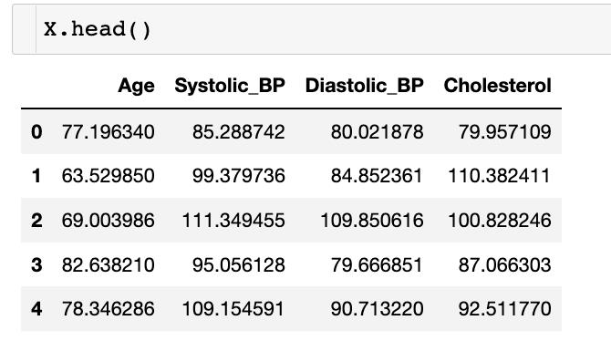
X 和 y 是 Pandas DataFrames，包含 6,000 名糖尿病患者的数据。

3 explore the dataset

The features (X) include the following fields:

• Age: (years)
• Systolic_BP: Systolic blood pressure (mmHg)收缩压
• Diastolic_BP: Diastolic blood pressure (mmHg)舒张压
• Cholesterol: (mg/DL) 胆固醇

target (y) 是患者是否发生视网膜病变的指标

• y = 1：患者患有视网膜病变。
• y = 0：患者没有视网膜病变。

在我们建立模型之前，让我们仔细看看我们的训练数据的分布。为此，我们将使用 75/25 拆分将数据拆分为训练集和测试集。

from sklearn.model_selection import train_test_split

X_train_raw, X_test_raw, y_train, y_test = train_test_split(X, y, train_size=0.75, random_state=0)

for col in X.columns:
    X_train_raw.loc[:, col].hist()
    plt.title(col)
    plt.show()

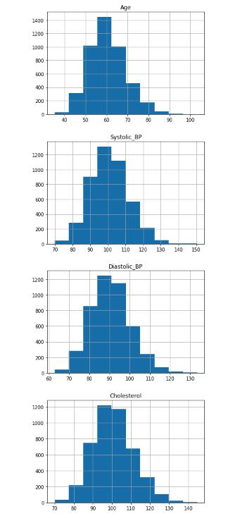
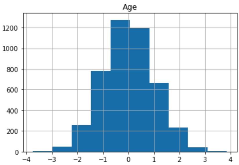
正如我们所看到的，这些分布通常呈钟形分布，但有轻微的向右偏斜。
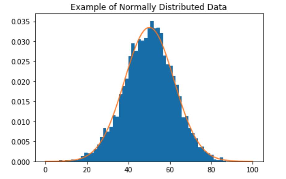
许多统计模型假设数据是正态分布的，形成一个对称的高斯钟形（没有偏斜），更像下面的例子。

我们可以通过消除偏斜将数据转换为更接近正态分布。消除偏斜的一种方法是将log函数应用于数据。让我们绘制特征变量的log，看看它是否产生了预期的效果。

for col in X_train_raw.columns:
    np.log(X_train_raw.loc[:, col]).hist()
    plt.title(col)
    plt.show()

这里使用了np.log()

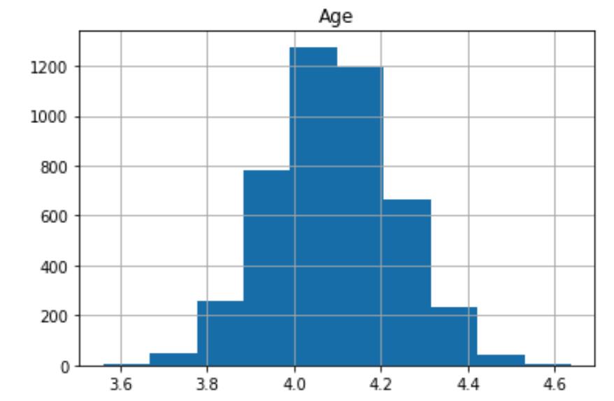
对比年龄的分布，取 log 后我们可以看到数据更加对称

4 Mean-Normalize the data

现在让我们 transform 我们的数据，使分布更接近标准正态分布。
首先，我们将使用 log 转换从分布中消除一些偏斜。然后我们将“标准化”分布，使其均值为零，标准差为 1。

编写一个函数，首先去除数据中的一些偏斜，然后标准化分布，以便对于每个数据点 $x$ ,
$$\overline{x}=\frac{x-mean(x)}{std(x)}$$
请注意，我们 test data 是“看不见的”数据。

• 这意味着我们不可能求到它的整体均值和方差，但可以使用训练数据来计算这些值，然后将它们用于标准化训练和测试数据。
• 更多讨论，请参阅这篇文章为什么我们需要重用训练参数来transform测试数据。

def make_standard_normal(df_train, df_test):
    """
    In order to make the data closer to a normal distribution, take log
    transforms to reduce the skew.
    Then standardize the distribution with a mean of zero and standard deviation of 1. 
  
    Args:
      df_train (dataframe): unnormalized training data.
      df_test (dataframe): unnormalized test data.
  
    Returns:
      df_train_normalized (dateframe): normalized training data.
      df_test_normalized (dataframe): normalized test data.
    """
    
    ### START CODE HERE (REPLACE INSTANCES OF 'None' with your code) ###  
    # Remove skew by applying the log function to the train set, and to the test set
    df_train_unskewed = np.log(df_train)
    df_test_unskewed = np.log(df_test)
    
    #calculate the mean and standard deviation of the training set
    mean = df_train_unskewed.mean(axis=0)
    stdev = df_train_unskewed.std(axis=0)
    
    # standardize the training set
    df_train_standardized = (df_train_unskewed - mean) / stdev
    
    # standardize the test set (see instructions and hints above)
    df_test_standardized = (df_test_unskewed - mean) / stdev
    
    ### END CODE HERE ###
    return df_train_standardized, df_test_standardized

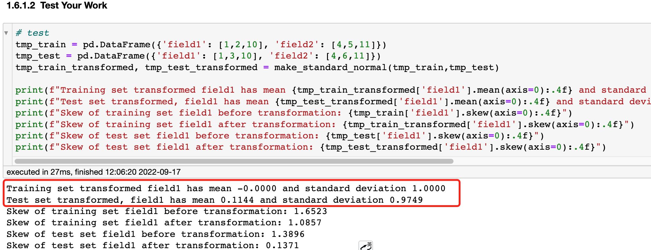
通过测试可以看到，经过标准化后，训练数据的均值为1，方差为0，测试数据集上虽然不是0和1，但也很接近。

把我们的X_train, X_test进行标准化

X_train, X_test = make_standard_normal(X_train_raw, X_test_raw)

经过数据转换后的数据分布👇

7 build the model

现在我们准备通过使用我们的数据训练逻辑回归来构建风险模型。

def lr_model(X_train, y_train):
    
    ### START CODE HERE (REPLACE INSTANCES OF 'None' with your code) ###
    # import the LogisticRegression class
    from sklearn.linear_model import LogisticRegression
    
    # create the model object
    model = LogisticRegression()
    
    # fit the model to the training data
    model.fit(X_train,y_train)
    
    ### END CODE HERE ###
    #return the fitted model
    return model

model_X = lr_model(X_train, y_train)

8 评估模型

我们使用c-index评估模型

• c-index 衡量风险评分的辨别力。
• 直观地说，较高的 c 指数表明模型的预测与一对患者的实际结果一致。
• c-index的公式是

KaTeX parse error: Undefined control sequence: \\mbox at position 2: \\̲m̲b̲o̲x̲cindex = \\fra…

• 允许的配对是一对具有不同结果（y=0和y=1）的患者。
• concordant配对是允许的配对，其中风险评分较高的患者也有较差的结果。
• ties 是允许配对中，其中患者具有相同的风险评分。

def cindex(y_true, scores):
    '''

    Input:
    y_true (np.array): a 1-D array of true binary outcomes (values of zero or one)
        0: patient does not get the disease
        1: patient does get the disease
    scores (np.array): a 1-D array of corresponding risk scores output by the model

    Output:
    c_index (float): (concordant pairs + 0.5*ties) / number of permissible pairs
    '''
    n = len(y_true)
    assert len(scores) == n

    concordant = 0
    permissible = 0
    ties = 0
    
    ### START CODE HERE (REPLACE INSTANCES OF 'None' with your code) ###
    # use two nested for loops to go through all unique pairs of patients
    for i in range(n):
        for j in range(i+1, n): #choose the range of j so that j>i
            
            # Check if the pair is permissible (the patient outcomes are different)
            if y_true[i] != y_true[j]:
                # Count the pair if it's permissible
                permissible =permissible + 1

                # For permissible pairs, check if they are concordant or are ties

                # check for ties in the score
                if scores[i] == scores[j]:
                    # count the tie
                    ties = ties + 1
                    # if it's a tie, we don't need to check patient outcomes, continue to the top of the for loop.
                    continue

                # case 1: patient i doesn't get the disease, patient j does
                if y_true[i] == 0 and y_true[j] == 1:
                    # Check if patient i has a lower risk score than patient j
                    if scores[i] < scores[j]:
                        # count the concordant pair
                        concordant = concordant + 1
                    # Otherwise if patient i has a higher risk score, it's not a concordant pair.
                    # Already checked for ties earlier

                # case 2: patient i gets the disease, patient j does not
                if y_true[i] == 1 and y_true[j] == 0:
                    # Check if patient i has a higher risk score than patient j
                    if scores[i] > scores[j]:
                        #count the concordant pair
                        concordant = concordant + 1
                    # Otherwise if patient i has a lower risk score, it's not a concordant pair.
                    # We already checked for ties earlier

    # calculate the c-index using the count of permissible pairs, concordant pairs, and tied pairs.
    c_index = (concordant + (0.5 * ties)) / permissible
    ### END CODE HERE ###
    
    return c_index

我们在上节课中，已经学习了c-index的理论基础，这里直接给代码，很好理解。

9 Evaluate the Model on the Test Set

使用 predict_proba 获得测试数据的概率。

scores = model_X.predict_proba(X_test)[:, 1]
c_index_X_test = cindex(y_test.values, scores)
print(f"c-index on test set is c_index_X_test:.4f")

out: c-index on test set is 0.8182

由于线性回归模型，每个特征都有自己的系数（coefficients），也可以理解为每个特征的权重，我们把系数画出来，看哪个特征对结果的影响更大

可以使用函数model.coef_计算系数

coeffs = pd.DataFrame(data = model_X.coef_, columns = X_train.columns)
coeffs.T.plot.bar(legend=None);

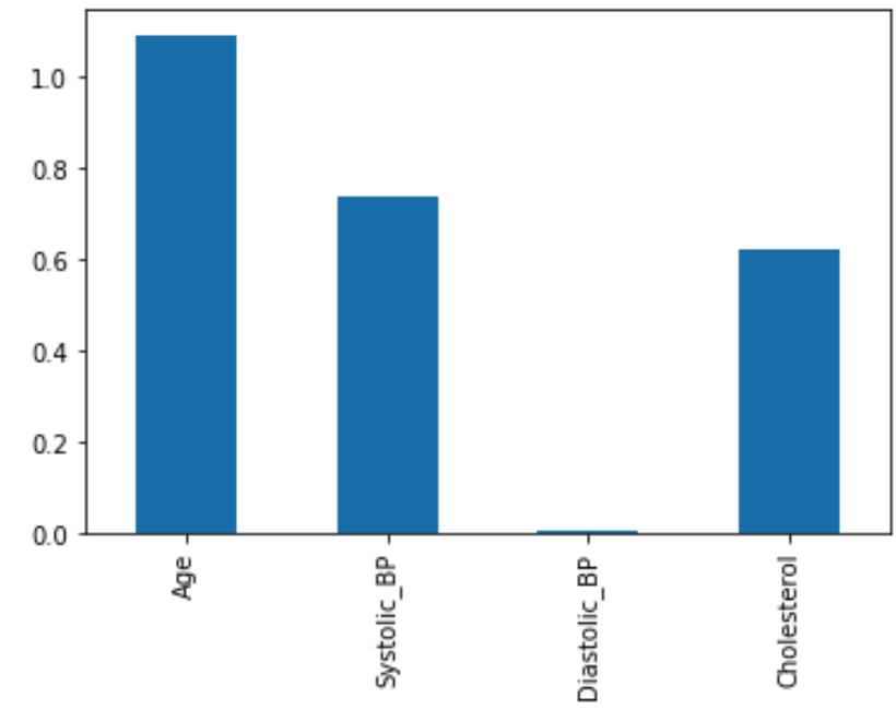
从图上可以看出，年龄对视网膜病变的影响最大。

10 Improve the Model

我们可以通过增加交互项改进模型

• For example, if we have data
  $$x=[x_1,x_2]$$
• We could add the product so that:
  $$\hat{x}=[x_1,x_2,x_1\ast x_2]$$

把所有的特征进行两两组合，使用乘法而不是加法（上一节课已经讨论过，为什么用乘法）

把组合后的特征都加入X_train中，重新训练模型。我们得到以下所有特征的系数，加入交互项后，c-index=0.8281,提升了一点一点性能。

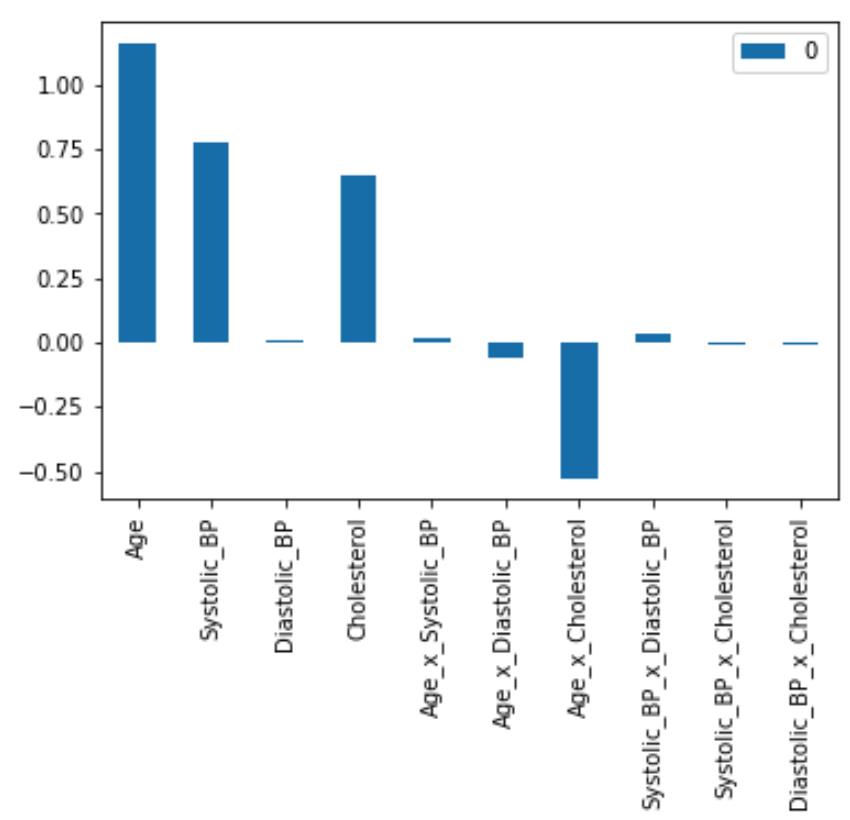
您可能会注意到 Age、Systolic_BP 和 Cholesterol 具有正系数。这意味着这三个特征的值越高，疾病的预测概率就越高。您还可能注意到年龄 x 胆固醇的交互作用具有负系数。这意味着年龄 x 胆固醇乘积的较高值会降低疾病的发病概率。

这部分代码略，详情自行下载。

文章持续更新，可以关注微信公众号【医学图像人工智能实战营】获取最新动态，一个关注于医学图像处理领域前沿科技的公众号。坚持已实践为主，手把手带你做项目，打比赛，写论文。凡原创文章皆提供理论讲解，实验代码，实验数据。只有实践才能成长的更快，关注我们，一起学习进步~

我是Tina, 我们下篇博客见~

白天工作晚上写文，呕心沥血

觉得写的不错的话最后，求点赞，评论，收藏。或者一键三连