pytorch-在竞赛中去摸索用法,用房价预测比赛了解数据处理流程
Posted 羞儿
tags:
篇首语:本文由小常识网(cha138.com)小编为大家整理,主要介绍了pytorch-在竞赛中去摸索用法,用房价预测比赛了解数据处理流程相关的知识,希望对你有一定的参考价值。
实战Kaggle比赛:房价预测
- 让我们动手实战一个Kaggle比赛:房价预测House Prices - Advanced Regression Techniques | Kaggle。本文将提供未经调优的数据的预处理、模型的设计和超参数的选择。通过动手操作、仔细观察实验现象、认真分析实验结果并不断调整方法,得到满意的结果。
获取和读取数据集
-
比赛数据分为训练数据集和测试数据集。两个数据集都包括每栋房子的特征,如街道类型、建造年份、房顶类型、地下室状况等特征值。这些特征值有连续的数字、离散的标签甚至是缺失值“na”。只有训练数据集包括了每栋房子的价格,也就是标签。可以访问比赛网页中的“Data”标签,并下载这些数据集。【You have accepted the rules for this competition. Good luck!】
-

-
将通过
pandas库读入并处理数据。 -
%matplotlib inline import torch import torch.nn as nn import numpy as np import pandas as pd print(torch.__version__) torch.set_default_tensor_type(torch.FloatTensor) train_data = pd.read_csv('./house-prices-advanced-regression-techniques/train.csv') test_data = pd.read_csv('./house-prices-advanced-regression-techniques/test.csv') print(train_data,test_data) -
1.13.1 Id MSSubClass MSZoning LotFrontage LotArea Street Alley LotShape \\ 0 1 60 RL 65.0 8450 Pave NaN Reg 1 2 20 RL 80.0 9600 Pave NaN Reg 2 3 60 RL 68.0 11250 Pave NaN IR1 3 4 70 RL 60.0 9550 Pave NaN IR1 4 5 60 RL 84.0 14260 Pave NaN IR1 ... ... ... ... ... ... ... ... ... 1455 1456 60 RL 62.0 7917 Pave NaN Reg 1456 1457 20 RL 85.0 13175 Pave NaN Reg 1457 1458 70 RL 66.0 9042 Pave NaN Reg 1458 1459 20 RL 68.0 9717 Pave NaN Reg 1459 1460 20 RL 75.0 9937 Pave NaN Reg LandContour Utilities ... PoolArea PoolQC Fence MiscFeature MiscVal \\ 0 Lvl AllPub ... 0 NaN NaN NaN 0 1 Lvl AllPub ... 0 NaN NaN NaN 0 2 Lvl AllPub ... 0 NaN NaN NaN 0 3 Lvl AllPub ... 0 NaN NaN NaN 0 4 Lvl AllPub ... 0 NaN NaN NaN 0 ... ... ... ... ... ... ... ... ... 1455 Lvl AllPub ... 0 NaN NaN NaN 0 1456 Lvl AllPub ... 0 NaN MnPrv NaN 0 1457 Lvl AllPub ... 0 NaN GdPrv Shed 2500 1458 Lvl AllPub ... 0 NaN NaN NaN 0 1459 Lvl AllPub ... 0 NaN NaN NaN 0 MoSold YrSold SaleType SaleCondition SalePrice 0 2 2008 WD Normal 208500 1 5 2007 WD Normal 181500 2 9 2008 WD Normal 223500 3 2 2006 WD Abnorml 140000 4 12 2008 WD Normal 250000 ... ... ... ... ... ... 1455 8 2007 WD Normal 175000 1456 2 2010 WD Normal 210000 1457 5 2010 WD Normal 266500 1458 4 2010 WD Normal 142125 1459 6 2008 WD Normal 147500 [1460 rows x 81 columns] Id MSSubClass MSZoning LotFrontage LotArea Street Alley LotShape \\ 0 1461 20 RH 80.0 11622 Pave NaN Reg 1 1462 20 RL 81.0 14267 Pave NaN IR1 2 1463 60 RL 74.0 13830 Pave NaN IR1 3 1464 60 RL 78.0 9978 Pave NaN IR1 4 1465 120 RL 43.0 5005 Pave NaN IR1 ... ... ... ... ... ... ... ... ... 1454 2915 160 RM 21.0 1936 Pave NaN Reg 1455 2916 160 RM 21.0 1894 Pave NaN Reg 1456 2917 20 RL 160.0 20000 Pave NaN Reg 1457 2918 85 RL 62.0 10441 Pave NaN Reg 1458 2919 60 RL 74.0 9627 Pave NaN Reg LandContour Utilities ... ScreenPorch PoolArea PoolQC Fence \\ 0 Lvl AllPub ... 120 0 NaN MnPrv 1 Lvl AllPub ... 0 0 NaN NaN 2 Lvl AllPub ... 0 0 NaN MnPrv 3 Lvl AllPub ... 0 0 NaN NaN 4 HLS AllPub ... 144 0 NaN NaN ... ... ... ... ... ... ... ... 1454 Lvl AllPub ... 0 0 NaN NaN 1455 Lvl AllPub ... 0 0 NaN NaN 1456 Lvl AllPub ... 0 0 NaN NaN 1457 Lvl AllPub ... 0 0 NaN MnPrv 1458 Lvl AllPub ... 0 0 NaN NaN MiscFeature MiscVal MoSold YrSold SaleType SaleCondition 0 NaN 0 6 2010 WD Normal 1 Gar2 12500 6 2010 WD Normal 2 NaN 0 3 2010 WD Normal 3 NaN 0 6 2010 WD Normal 4 NaN 0 1 2010 WD Normal ... ... ... ... ... ... ... 1454 NaN 0 6 2006 WD Normal 1455 NaN 0 4 2006 WD Abnorml 1456 NaN 0 9 2006 WD Abnorml 1457 Shed 700 7 2006 WD Normal 1458 NaN 0 11 2006 WD Normal [1459 rows x 80 columns] -
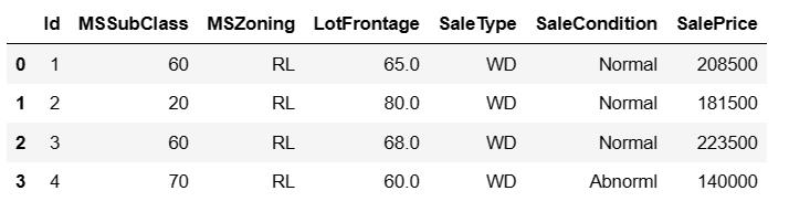
查看前4个样本的前4个特征、后2个特征和标签(SalePrice):
-
可以看到第一个特征是Id,它能帮助模型记住每个训练样本,但难以推广到测试样本,所以我们不使用它来训练。我们将所有的训练数据和测试数据的79个特征按样本连结。
-
all_features = pd.concat((train_data.iloc[:, 1:-1], test_data.iloc[:, 1:]))
预处理数据
-
对连续数值的特征做标准化(standardization):设该特征在整个数据集上的均值为 μ \\mu μ,标准差为 σ \\sigma σ。那么,我们可以将该特征的每个值先减去 μ \\mu μ再除以 σ \\sigma σ得到标准化后的每个特征值。对于缺失的特征值,将其替换成该特征的均值。
-
numeric_features = all_features.dtypes[all_features.dtypes != 'object'].index all_features[numeric_features] = all_features[numeric_features].apply(lambda x: (x - x.mean()) / (x.std())) # 标准化后,每个数值特征的均值变为0,所以可以直接用0来替换缺失值 all_features[numeric_features] = all_features[numeric_features].fillna(0) -
接下来将离散数值转成指示特征。举个例子,假设特征MSZoning里面有两个不同的离散值RL和RM,那么这一步转换将去掉MSZoning特征,并新加两个特征MSZoning_RL和MSZoning_RM,其值为0或1。如果一个样本原来在MSZoning里的值为RL,那么有MSZoning_RL=1且MSZoning_RM=0。
-
# dummy_na=True将缺失值也当作合法的特征值并为其创建指示特征 all_features = pd.get_dummies(all_features, dummy_na=True) all_features.shape # (2919, 331) -
可以看到这一步转换将特征数从79增加到了331。最后,通过
values属性得到NumPy格式的数据,并转成Tensor方便后面的训练。 -
n_train = train_data.shape[0]
train_features = torch.tensor(all_features[:n_train].values, dtype=torch.float)
test_features = torch.tensor(all_features[n_train:].values, dtype=torch.float)
train_labels = torch.tensor(train_data.SalePrice.values, dtype=torch.float).view(-1, 1)
训练模型
-
使用一个基本的线性回归模型和平方损失函数来训练模型。下面定义比赛用来评价模型的对数均方根误差。给定预测值 y ^ 1 , … , y ^ n \\hat y_1, \\ldots, \\hat y_n y^1,…,y^n和对应的真实标签 y 1 , … , y n y_1,\\ldots, y_n y1,…,yn,它的定义为 1 n ∑ i = 1 n ( log ( y i ) − log ( y ^ i ) ) 2 \\sqrt\\frac1n\\sum_i=1^n\\left(\\log(y_i)-\\log(\\hat y_i)\\right)^2 n1∑i=1n(log(yi)−log(y^i))2.对数均方根误差的实现如下。
-
loss = torch.nn.MSELoss() def get_net(feature_num): net = nn.Linear(feature_num, 1) for param in net.parameters(): nn.init.normal_(param, mean=0, std=0.01) return net def log_rmse(net, features, labels): with torch.no_grad(): # 将小于1的值设成1,使得取对数时数值更稳定 clipped_preds = torch.max(net(features), torch.tensor(1.0)) rmse = torch.sqrt(loss(clipped_preds.log(), labels.log())) return rmse.item() -
下面的训练函数跟本章中前几节的不同在于使用了Adam优化算法。相对之前使用的小批量随机梯度下降,它对学习率相对不那么敏感。
-
def train(net, train_features, train_labels, test_features, test_labels,
          num_epochs, learning_rate, weight_decay, batch_size):
    train_ls, test_ls = [], []
    dataset = torch.utils.data.TensorDataset(train_features, train_labels)
    train_iter = torch.utils.data.DataLoader(dataset, batch_size, shuffle=True)
    # 这里使用了Adam优化算法
    optimizer = torch.optim.Adam(params=net.parameters(), lr=learning_rate, weight_decay=weight_decay)
    net = net.float()
    for epoch in range(num_epochs):
        for X, y in train_iter:
            l = loss(net(X.float()), y.float())
            optimizer.zero_grad()
            l.backward()
            optimizer.step()
        train_ls.append(log_rmse(net, train_features, train_labels))
        if test_labels is not None:
            test_ls.append(log_rmse(net, test_features, test_labels))
    return train_ls, test_ls
K折交叉验证
-
它将被用来选择模型设计并调节超参数。下面实现了一个函数,它返回第
i折交叉验证时所需要的训练和验证数据。在K折交叉验证中我们训练K次并返回训练和验证的平均误差。 -
from IPython import display from matplotlib import pyplot as plt def use_svg_display(): # 用矢量图显示 display.display_svg() def set_figsize(figsize=(3.5, 2.5)): use_svg_display() # 设置图的尺寸 plt.rcParams['figure.figsize'] = figsize def semilogy(x_vals, y_vals, x_label, y_label, x2_vals=None, y2_vals=None, legend=None, figsize=(3.5, 2.5)): set_figsize(figsize) plt.xlabel(x_label) plt.ylabel(y_label) plt.semilogy(x_vals, y_vals) if x2_vals and y2_vals: plt.semilogy(x2_vals, y2_vals, linestyle=':') plt.legend(legend) def get_k_fold_data(k, i, X, y): # 返回第i折交叉验证时所需要的训练和验证数据 assert k > 1 fold_size = X.shape[0] // k X_train, y_train = None, None for j in range(k): idx = slice(j * fold_size, (j + 1) * fold_size) X_part, y_part = X[idx, :], y[idx] if j == i: X_valid, y_valid = X_part, y_part elif X_train is None: X_train, y_train = X_part, y_part else: X_train = torch.cat((X_train, X_part), dim=0) y_train = torch.cat((y_train, y_part), dim=0) return X_train, y_train, X_valid, y_valid def k_fold(k, X_train, y_train, num_epochs,learning_rate, weight_decay, batch_size): train_l_sum, valid_l_sum = 0, 0 for i in range(k): data = get_k_fold_data(k, i, X_train, y_train) net = get_net(X_train.shape[1]) train_ls, valid_ls = train(net,小白学习之pytorch框架之实战Kaggle比赛:房价预测(K折交叉验证*args**kwargs)
本篇博客代码来自于《动手学深度学习》pytorch版,也是代码较多,解释较少的一篇。不过好多方法在我以前的博客都有提,所以这次没提。还有一个原因是,这篇博客的代码,只要好好看看肯定能看懂(前提是python语法大概了解),这是我不加很多解释的重要原因。
K折交叉验证实现
def get_k_fold_data(k, i, X, y): # 返回第i折交叉验证时所需要的训练和验证数据,分开放,X_train为训练数据,X_valid为验证数据 assert k > 1 fold_size = X.shape[0] // k # 双斜杠表示除完后再向下取整 X_train, y_train = None, None for j in range(k): idx = slice(j * fold_size, (j + 1) * fold_size) #slice(start,end,step)切片函数 X_part, y_part = X[idx, :], y[idx] if j == i: X_valid, y_valid = X_part, y_part elif X_train is None: X_train, y_train = X_part, y_part else: X_train = torch.cat((X_train, X_part), dim=0) #dim=0增加行数,竖着连接 y_train = torch.cat((y_train, y_part), dim=0) return X_train, y_train, X_valid, y_valid def k_fold(k, X_train, y_train, num_epochs,learning_rate, weight_decay, batch_size): train_l_sum, valid_l_sum = 0, 0 for i in range(k): data = get_k_fold_data(k, i, X_train, y_train) # 获取k折交叉验证的训练和验证数据 net = get_net(X_train.shape[1]) #get_net在这是一个基本的线性回归模型,方法实现见附录1 train_ls, valid_ls = train(net, *data, num_epochs, learning_rate, weight_decay, batch_size) #train方法见后面附录2 train_l_sum += train_ls[-1] valid_l_sum += valid_ls[-1] if i == 0: d2l.semilogy(range(1, num_epochs + 1), train_ls, ‘epochs‘, ‘rmse‘, range(1, num_epochs + 1), valid_ls, [‘train‘, ‘valid‘]) #画图,且是对y求对数了,x未变。方法实现见附录3 print(‘fold %d, train rmse %f, valid rmse %f‘ % (i, train_ls[-1], valid_ls[-1])) return train_l_sum / k, valid_l_sum / k*args:表示接受任意长度的参数,然后存放入一个元组中;如def fun(*args) print(args),‘fruit‘,‘animal‘,‘human‘作为参数传进去,输出(‘fruit‘,‘animal‘,‘human‘)
**kwargs:表示接受任意长的参数,然后存放入一个字典中;如
def fun(**kwargs): for key, value in kwargs.items(): print("%s:%s" % (key,value)fun(a=1,b=2,c=3)会输出 a=1 b=2 c=3
附录1
loss = torch.nn.MSELoss() def get_net(feature_num): net = nn.Linear(feature_num, 1) for param in net.parameters(): nn.init.normal_(param, mean=0, std=0.01) return net附录2
def train(net, train_features, train_labels, test_features, test_labels, num_epochs, learning_rate,weight_decay, batch_size): train_ls, test_ls = [], [] dataset = torch.utils.data.TensorDataset(train_features, train_labels) train_iter = torch.utils.data.DataLoader(dataset, batch_size, shuffle=True) #TensorDataset和DataLoader的使用请查看我以前的博客 #这里使用了Adam优化算法 optimizer = torch.optim.Adam(params=net.parameters(), lr= learning_rate, weight_decay=weight_decay) net = net.float() for epoch in range(num_epochs): for X, y in train_iter: l = loss(net(X.float()), y.float()) optimizer.zero_grad() l.backward() optimizer.step() train_ls.append(log_rmse(net, train_features, train_labels)) if test_labels is not None: test_ls.append(log_rmse(net, test_features, test_labels)) return train_ls, test_ls附录3
def semilogy(x_vals, y_vals, x_label, y_label, x2_vals=None, y2_vals=None, legend=None, figsize=(3.5, 2.5)): set_figsize(figsize) plt.xlabel(x_label) plt.ylabel(y_label) plt.semilogy(x_vals, y_vals) if x2_vals and y2_vals: plt.semilogy(x2_vals, y2_vals, linestyle=‘:‘) plt.legend(legend)注:由于最近有其他任务,所以此博客写的匆忙,等我有时间后会丰富,也可能加详细解释。
以上是关于pytorch-在竞赛中去摸索用法,用房价预测比赛了解数据处理流程的主要内容,如果未能解决你的问题,请参考以下文章