系统生物学大肠杆菌蛋白互作网络分析（系统与合成生物学第三次作业）

Posted 2023-03-29 Dream of Grass

摘要

下载大肠杆菌蛋白互作网络（Ecoli PPI network）数据，使用Python对大肠杆菌蛋白互作网络进行筛选，并使用Cytoscape进行圆形布局可视化。此外，还绘制度分布函数并用幂函数进行拟合。

大肠杆菌蛋白互作网络

数据下载

我们从string（https://cn.string-db.org/）中下载ppi数据。

• 大肠杆菌蛋白互作网络下载地址：https://stringdb-static.org/download/protein.links.v11.5/511145.protein.links.v11.5.txt.gz
• 蛋白质信息下载地址：https://stringdb-static.org/download/protein.info.v11.5/511145.protein.info.v11.5.txt.gz

数据处理

将蛋白质的原始id转换为蛋白质名，并筛选结合分数大于800的蛋白质对。

import pandas as pd
import networkx as nx

# 处理Ecoli的ppi数据
filepath = "D:/000大三下/系统与合成生物学/"
link_filename = '511145.protein.links.v11.5.txt'
info_filename = '511145.protein.info.v11.5.txt'
ppi_link = pd.read_csv(filepath + link_filename, sep=' ', header=0)
ppi_info = pd.read_csv(filepath + info_filename, sep='\\t', header=0)
# 筛选结合分数大于800的protein pair
ppi_link = ppi_link[ppi_link['combined_score'] > 800]
# 把stiring_protein_id替换成preferred_name
ppi = pd.merge(ppi_link, ppi_info[['#string_protein_id', 'preferred_name']], left_on='protein1',
               right_on='#string_protein_id')
ppi = pd.merge(ppi, ppi_info[['#string_protein_id', 'preferred_name']], left_on='protein2',
               right_on='#string_protein_id')
ppi = ppi[['preferred_name_x', 'preferred_name_y', 'combined_score']]
ppi.columns = ['protein1', 'protein2', 'combined_score']
# 保存
ppi.to_csv(filepath + 'Ecoli_ppi.csv', index=False, header=1)

处理后的数据如下：

表1 处理后的蛋白互作网络

protein1	protein2	combined_score
thrA	dapA	945
dapB	dapA	999
dapD	dapA	966
dapE	dapA	948
bamC	dapA	945
lysA	dapA	984
asd	dapA	994
dapF	dapA	968
metL	dapA	938
lysC	dapA	858

圆形布局可视化蛋白互作网络

图1 蛋白互作网络全貌 图2 蛋白互作网络微观

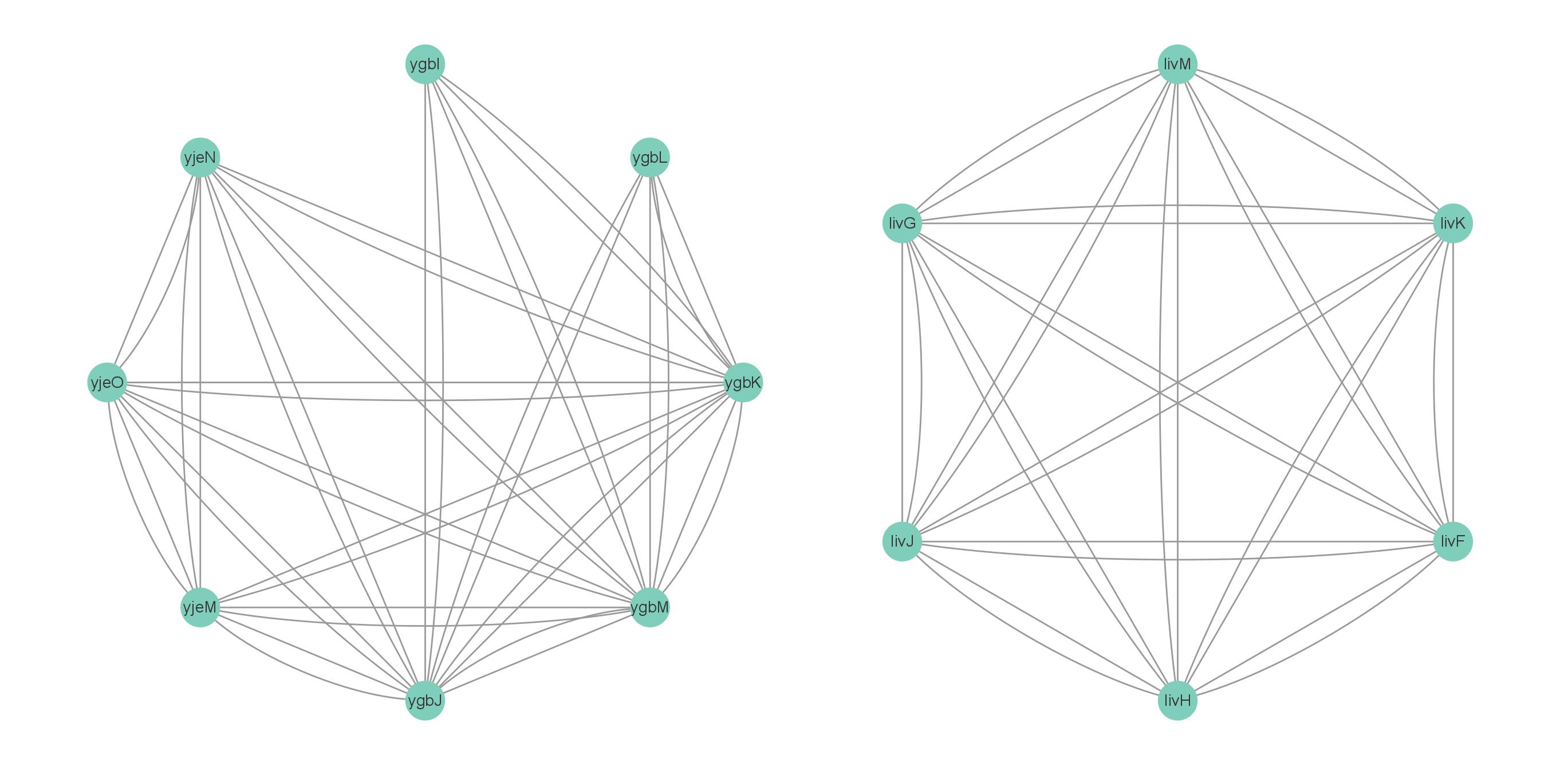
计算中心性指标

使用networkx，计算Degree Centrality、Closeness Centrality、Betweenness Centrality和Eigenvector Centrality。计算结束后对其求和并降序排列。

net = ppi[['protein1', 'protein2']]
net.drop_duplicates()
G = nx.from_pandas_edgelist(net, "protein1", "protein2")
# 计算中心性
degree_centrality = nx.degree_centrality(G)
closeness_centrality = nx.closeness_centrality(G)
betweenness_centrality = nx.betweenness_centrality(G)
eigenvector_centrality = nx.eigenvector_centrality(G)
# 将指标转换为DataFrame格式
centrality_df = pd.DataFrame('Degree Centrality': degree_centrality,
                              'Closeness Centrality': closeness_centrality,
                              'Betweenness Centrality': betweenness_centrality,
                              'Eigenvector Centrality': eigenvector_centrality)
# 求和并排序
centrality_df['Sum'] = centrality_df.sum(axis=1)
centrality_df = centrality_df.sort_values(by='Sum', ascending=False)
# 保存
centrality_df.to_csv(filepath + 'Ecoli_ppi_centrality.csv')

表2 蛋白互作网络中心性指标

Protein	Degree Centrality	Closeness Centrality	Betweenness Centrality	Eigenvector Centrality	Sum
rpoB	0.032583	0.274943	0.018549	0.105043	0.431118
rpsL	0.029222	0.260888	0.011465	0.115507	0.417082
rplB	0.029222	0.261492	0.00294	0.121612	0.415266
rpmA	0.027411	0.263495	0.006903	0.117347	0.415155
rplM	0.029222	0.25926	0.002129	0.121699	0.41231
rplE	0.028963	0.257817	0.002343	0.122201	0.411324
rpsB	0.027929	0.260983	0.002664	0.117817	0.409392
rplD	0.028187	0.256263	0.001058	0.122461	0.407969
rplV	0.027929	0.255628	0.001112	0.121178	0.405846
rplC	0.02767	0.255719	0.00102	0.12137	0.405779

绘制度分布函数并用幂函数拟合

使用python进行绘制并拟合。幂指数为-0.599。

# 计算度分布函数
# 即每个度数对应的节点数除以总节点数。
degree_sequence = sorted([d for n, d in G.degree()], reverse=True)
degree_count = np.zeros(max(degree_sequence)+1)
for degree in degree_sequence:
    degree_count[degree] += 1
degree_distribution = degree_count/sum(degree_count)

# 绘制度分布函数的双对数轴图
x = np.arange(1, len(degree_distribution)+1)
y = degree_distribution
# plt.loglog(x, y, color = 'chocolate', marker = '.')
plt.plot(x, y, color = 'chocolate', marker = '.')
# 使用幂函数拟合，计算幂指数的值
def power_law(x, a, b):
    return a * x ** (b)

popt, pcov = curve_fit(power_law, x, y)
a, b = popt
# plt.loglog(x, power_law(x, a, b), 'c--', label='fit: y=%5.3f*x^(%5.3f)' % (a, b))
plt.plot(x, power_law(x, a, b), 'c--', label='fit: y=%5.3f*x^(%5.3f)' % (a, b))
plt.xlabel('Degree)')
plt.ylabel('Frequency)')
# plt.xlabel('log(Degree)')
# plt.ylabel('log(Frequency)')
plt.legend()
plt.savefig(filepath+'Degree_distribution.png')
plt.show()
print('幂指数的值为：', b)

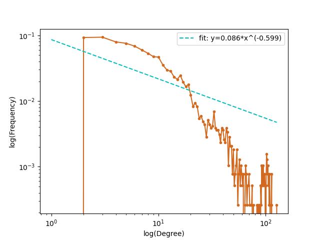图3 横纵坐标对数转换前	图4 横纵坐标对数转换后

完整代码

# _*_ coding: utf-8 _*_
# @Time : 2023-03-28 23:03 
# @Author : YingHao Zhang(池塘春草梦)
# @Version：v0.1
# @File : network.py
# @desc : 系统与合成生物学作业。读取Ecoli的ppi数据，将蛋白质的原始id转换为蛋白质名，并计算四种中心性指标。输入：ppi的link和info文件。输出：①处理后的ppi网络（包括蛋白质对和结合分数）；②蛋白质的四种中心性指标和四种中心性指标的和。绘制度分布曲线，并用幂函数拟合。

import pandas as pd
import networkx as nx
import time

start_time = time.time()
# 处理Ecoli的ppi数据
filepath = "D:/000大三下/系统与合成生物学/"
link_filename = '511145.protein.links.v11.5.txt'
info_filename = '511145.protein.info.v11.5.txt'
ppi_link = pd.read_csv(filepath + link_filename, sep=' ', header=0)
ppi_info = pd.read_csv(filepath + info_filename, sep='\\t', header=0)
# 筛选结合分数大于800的protein pair
ppi_link = ppi_link[ppi_link['combined_score'] > 800]
# 把stiring_protein_id替换成preferred_name
ppi = pd.merge(ppi_link, ppi_info[['#string_protein_id', 'preferred_name']], left_on='protein1',
               right_on='#string_protein_id')
ppi = pd.merge(ppi, ppi_info[['#string_protein_id', 'preferred_name']], left_on='protein2',
               right_on='#string_protein_id')
ppi = ppi[['preferred_name_x', 'preferred_name_y', 'combined_score']]
ppi.columns = ['protein1', 'protein2', 'combined_score']
# 保存
ppi.to_csv(filepath + 'Ecoli_ppi.csv', index=False, header=1)
net = ppi[['protein1', 'protein2']]
net.drop_duplicates()
G = nx.from_pandas_edgelist(net, "protein1", "protein2")
# 计算中心性
degree_centrality = nx.degree_centrality(G)
closeness_centrality = nx.closeness_centrality(G)
betweenness_centrality = nx.betweenness_centrality(G)
eigenvector_centrality = nx.eigenvector_centrality(G)
# 将指标转换为DataFrame格式
centrality_df = pd.DataFrame('Degree Centrality': degree_centrality,
                              'Closeness Centrality': closeness_centrality,
                              'Betweenness Centrality': betweenness_centrality,
                              'Eigenvector Centrality': eigenvector_centrality)
# 求和并排序
centrality_df['Sum'] = centrality_df.sum(axis=1)
centrality_df = centrality_df.sort_values(by='Sum', ascending=False)
# 保存
centrality_df.to_csv(filepath + 'Ecoli_ppi_centrality.csv')

import numpy as np
import matplotlib.pyplot as plt
from scipy.optimize import curve_fit

# 计算度分布函数
# 即每个度数对应的节点数除以总节点数。
degree_sequence = sorted([d for n, d in G.degree()], reverse=True)
degree_count = np.zeros(max(degree_sequence)+1)
for degree in degree_sequence:
    degree_count[degree] += 1
degree_distribution = degree_count/sum(degree_count)

# 绘制度分布函数的双对数轴图
x = np.arange(1, len(degree_distribution)+1)
y = degree_distribution
# plt.loglog(x, y, color = 'chocolate', marker = '.')
plt.plot(x, y, color = 'chocolate', marker = '.')
# 使用幂函数拟合，计算幂指数的值
def power_law(x, a, b):
    return a * x ** (b)

popt, pcov = curve_fit(power_law, x, y)
a, b = popt
# plt.loglog(x, power_law(x, a, b), 'c--', label='fit: y=%5.3f*x^(%5.3f)' % (a, b))
plt.plot(x, power_law(x, a, b), 'c--', label='fit: y=%5.3f*x^(%5.3f)' % (a, b))
plt.xlabel('Degree)')
plt.ylabel('Frequency)')
# plt.xlabel('log(Degree)')
# plt.ylabel('log(Frequency)')
plt.legend()
plt.savefig(filepath+'Degree_distribution.png')
plt.show()

print('幂指数的值为：', b)

end_time = time.time()
run_time = end_time - start_time
print("Done (/▽＼)")
print("代码运行时间为：分秒".format(int(run_time / 60), round(run_time % 60)))