对保存的vgg16.ckpt模型实现特征图可视化

Posted 2022-12-02 大彤小忆

  在使用NWPU VHR-10数据集训练Faster R-CNN模型之后，可以通过对保存的模型实现特征图可视化来进一步分析模型。

  在训练结束后，我们会将一组模型复制到./output/vgg16/voc_2007_trainval/default路径下进行测试。

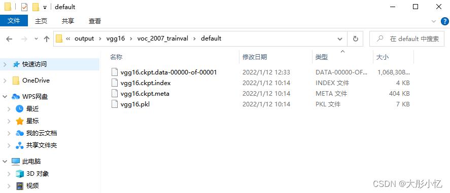
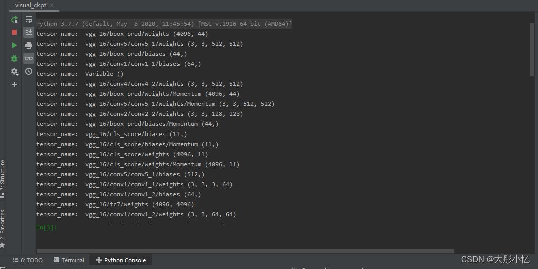
  在对特征图进行可视化前，首先新建一个visual_ckpt.py文件查看vgg16.ckpt文件的内容、参数名称及尺寸，具体代码如下所示。

from tensorflow.python import pywrap_tensorflow

checkpoint_path = 'E:/Remote Sensing/Faster-RCNN_for_NWPU VHR-10/output/vgg16/voc_2007_trainval/default/vgg16.ckpt'

reader = pywrap_tensorflow.NewCheckpointReader(checkpoint_path)  # tf.train.NewCheckpointReader
var_to_shape_map = reader.get_variable_to_shape_map()
for key in var_to_shape_map:
    print("tensor_name: ", key, reader.get_tensor(key).shape)

  运行代码后得到的结果如下图所示。

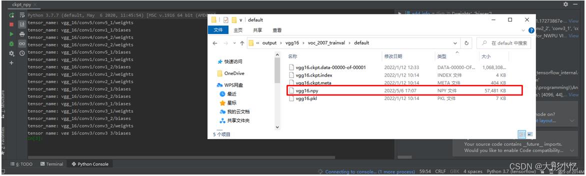
  然后新建一个ckpt_npy.py文件将vgg16.ckpt文件转为vgg16.npy文件，具体代码如下所示。

import numpy as np
import tensorflow as tf
from tensorflow.python import pywrap_tensorflow

checkpoint_path = 'E:/Remote Sensing/Faster-RCNN_for_NWPU VHR-10/output/vgg16/voc_2007_trainval/default/vgg16.ckpt'  # your ckpt path
reader = pywrap_tensorflow.NewCheckpointReader(checkpoint_path)
var_to_shape_map = reader.get_variable_to_shape_map()

alexnet = 
alexnet_layer = ['conv1_1', 'conv1_2', 'conv2_1', 'conv2_2', 'conv3_1', 'conv3_2', 'conv3_3', 'conv4_1', 'conv4_2', 'conv4_3', 'conv5_1', 'conv5_2', 'conv5_3']

add_info = ['weights', 'biases']

alexnet = 'conv1_1': [[], []], 'conv1_2': [[], []], 'conv2_1': [[], []], 'conv2_2': [[], []], 'conv3_1': [[], []], 'conv3_2': [[], []], 'conv3_3': [[], []], 'conv4_1': [[], []], 'conv4_2': [[], []], 'conv4_3': [[], []], 'conv5_1': [[], []], 'conv5_2': [[], []], 'conv5_3': [[], []]

for key in var_to_shape_map:
    str_name = key
    if str_name.find('Momentum') > -1:
        continue
    if str_name.find('Variable') > -1:
        continue
    if str_name.find('rpn') > -1:
        continue
    if str_name.find('bbox') > -1:
        continue
    if str_name.find('cls') > -1:
        continue
    if str_name.find('fc') > -1:
        continue
    print('tensor_name:', str_name)

    if str_name.find('/') > -1:
        names = str_name.split('/')
        # first layer name and weight, bias
        if len(names) > 3:
            layer_name = names[2]
            layer_add_info = names[3]
    else:
        layer_name = str_name
        layer_add_info = None

    if layer_add_info == 'weights':
         alexnet[layer_name][0] = reader.get_tensor(key)
    elif layer_add_info == 'biases':
        alexnet[layer_name][1] = reader.get_tensor(key)
    else:
         alexnet[layer_name] = reader.get_tensor(key)

# save npy
np.save('E:/Remote Sensing/Faster-RCNN_for_NWPU VHR-10/output/vgg16/voc_2007_trainval/default/vgg16.npy', alexnet)
print('save npy over...')

  运行代码后得到的结果如下图所示，可以在./output/vgg16/voc_2007_trainval/default路径下得到vgg16.npy文件。

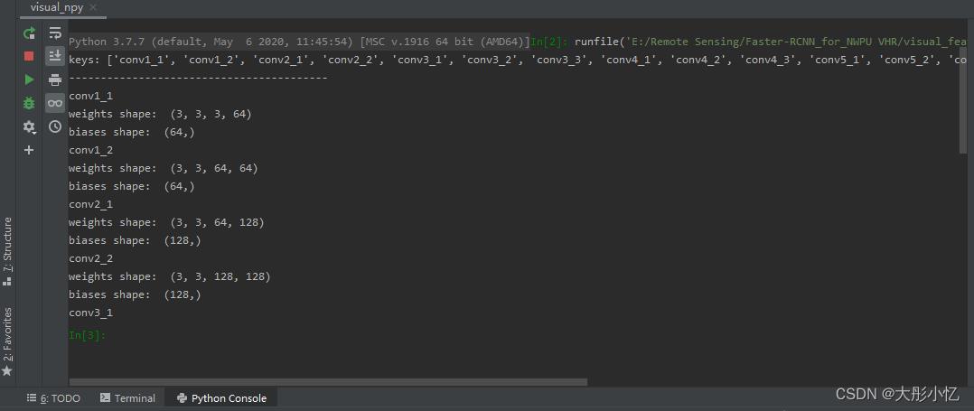
  接下来新建一个visual_npy.py文件查看vgg16.npy文件的参数，具体代码如下所示。

import numpy as np

data_dict = np.load('E:/Remote Sensing/Faster-RCNN_for_NWPU VHR-10/output/vgg16/voc_2007_trainval/default/vgg16.npy', encoding='latin1', allow_pickle=True).item()

keys = sorted(data_dict.keys())
# keys: 即为卷积层和全连接层的变量名
print("keys:", keys)
print("-----------------------------------------")

for key in keys:
    weights = data_dict[key][0]
    biases = data_dict[key][1]
    print(key)
    print('weights shape: ', weights.shape)
    print('biases shape: ', biases.shape)

  运行代码后得到的结果如下图所示。

  最后新建一个visual_feature.py文件对特征提取网络VGG16实现特征图可视化。

import numpy as np
import tensorflow as tf
import time
from PIL import Image
import matplotlib.pyplot as plt

# VGG 自带的一个常量，之前VGG训练通过归一化，所以现在同样需要作此操作
VGG_MEAN = [102.9801, 115.9465, 122.7717]  # rgb 三通道的均值

class VGGNet():
    '''
    创建 vgg16 网络 结构
    从模型中载入参数
    '''

    def __init__(self, data_dict):
        '''
        传入vgg16模型
        :param data_dict: vgg16.npy (字典类型)
        '''
        self.data_dict = data_dict

    def get_conv_filter(self, name):
        '''
        得到对应名称的卷积层
        :param name: 卷积层名称
        :return: 该卷积层输出
        '''
        return tf.constant(self.data_dict[name][0], name='conv')

    def get_fc_weight(self, name):
        '''
        获得名字为name的全连接层权重
        :param name: 连接层名称
        :return: 该层权重
        '''
        return tf.constant(self.data_dict[name][0], name='fc')

    def get_bias(self, name):
        '''
        获得名字为name的全连接层偏置
        :param name: 连接层名称
        :return: 该层偏置
        '''
        return tf.constant(self.data_dict[name][1], name='bias')

    def conv_layer(self, x, name):
        '''
        创建一个卷积层
        :param x:
        :param name:
        :return:
        '''
        # 在写计算图模型的时候，加一些必要的 name_scope，这是一个比较好的编程规范
        # 可以防止命名冲突， 二可视化计算图的时候比较清楚
        with tf.name_scope(name):
            # 获得 w 和 b
            conv_w = self.get_conv_filter(name)
            conv_b = self.get_bias(name)

            # 进行卷积计算
            h = tf.nn.conv2d(x, conv_w, strides=[1, 1, 1, 1], padding='SAME')
            '''
            因为此刻的 w 和 b 是从外部传递进来，所以使用 tf.nn.conv2d()
            tf.nn.conv2d(input, filter, strides, padding, use_cudnn_on_gpu = None, name = None) 参数说明：
            input 输入的tensor， 格式[batch, height, width, channel]
            filter 卷积核 [filter_height, filter_width, in_channels, out_channels] 
                分别是：卷积核高，卷积核宽，输入通道数，输出通道数
            strides 步长 卷积时在图像每一维度的步长，长度为4
            padding 参数可选择 “SAME” “VALID”

            '''
            # 加上偏置
            h = tf.nn.bias_add(h, conv_b)
            # 使用激活函数
            h = tf.nn.relu(h)
            return h

    def pooling_layer(self, x, name):
        '''
        创建池化层
        :param x: 输入的tensor
        :param name: 池化层名称
        :return: tensor
        '''
        return tf.nn.max_pool(x,
                              ksize=[1, 2, 2, 1],  # 核参数， 注意：都是4维
                              strides=[1, 2, 2, 1],
                              padding='SAME',
                              name=name
                              )

    def fc_layer(self, x, name, activation=tf.nn.relu):
        '''
        创建全连接层
        :param x: 输入tensor
        :param name: 全连接层名称
        :param activation: 激活函数名称
        :return: 输出tensor
        '''
        with tf.name_scope(name, activation):
            # 获取全连接层的 w 和 b
            fc_w = self.get_fc_weight(name)
            fc_b = self.get_bias(name)
            # 矩阵相乘 计算
            h = tf.matmul(x, fc_w)
            # 　添加偏置
            h = tf.nn.bias_add(h, fc_b)
            # 因为最后一层是没有激活函数relu的，所以在此要做出判断
            if activation is None:
                return h
            else:
                return activation(h)

    def flatten_layer(self, x, name):
        '''
        展平
        :param x: input_tensor
        :param name:
        :return: 二维矩阵
        '''
        with tf.name_scope(name):
            # [batch_size, image_width, image_height, channel]
            x_shape = x.get_shape().as_list()
            # 计算后三维合并后的大小
            dim = 1
            for d in x_shape[1:]:
                dim *= d
            # 形成一个二维矩阵
            x = tf.reshape(x, [-1, dim])
            return x

    def build(self, x_rgb):
        '''
        创建vgg16 网络
        :param x_rgb: [1, 224, 224, 3]
        :return:
        '''
        start_time = time.time()
        print('模型开始创建……')
        # 将输入图像进行处理，将每个通道减去均值
        r, g, b = tf.split(x_rgb, [1, 1, 1], axis=3)
        '''
        tf.split(value, num_or_size_split, axis=0)用法：
        value:输入的Tensor
        num_or_size_split:有两种用法：
            1.直接传入一个整数，代表会被切成几个张量，切割的维度有axis指定
            2.传入一个向量，向量长度就是被切的份数。传入向量的好处在于，可以指定每一份有多少元素
        axis, 指定从哪一个维度切割
        因此，上一句的意思就是从第4维切分，分为3份，每一份只有1个元素
        '''
        # 将 处理后的通道再次合并起来
        x_bgr = tf.concat([b - VGG_MEAN[0], g - VGG_MEAN[1], r - VGG_MEAN[2]], axis=3)

        # 开始构建卷积层（下面这些变量名称不能乱取，必须要和vgg16模型保持一致）
        self.conv1_1 = self.conv_layer(x_bgr, 'conv1_1')
        self.conv1_2 = self.conv_layer(self.conv1_1, 'conv1_2')
        self.pool1 = self.pooling_layer(self.conv1_2, 'pool1')

        self.conv2_1 = self.conv_layer(self.pool1, 'conv2_1')
        self.conv2_2 = self.conv_layer(self.conv2_1, 'conv2_2')
        self.pool2 = self.pooling_layer(self.conv2_2, 'pool2')

        self.conv3_1 = self.conv_layer(self.pool2, 'conv3_1')
        self.conv3_2 = self.conv_layer(self.conv3_1, 'conv3_2')
        self.conv3_3 = self.conv_layer(self.conv3_2, 'conv3_3')
        self.pool3 = self.pooling_layer(self.conv3_3, 'pool3')

        self.conv4_1 = self.conv_layer(self.pool3, 'conv4_1')
        self.conv4_2 = self.conv_layer(self.conv4_1, 'conv4_2')
        self.conv4_3 = self.conv_layer(self.conv4_2, 'conv4_3')
        self.pool4 = self.pooling_layer(self.conv4_3, 'pool4')

        self.conv5_1 = self.conv_layer(self.pool4, 'conv5_1')
        self.conv5_2 = self.conv_layer(self.conv5_1, 'conv5_2')
        self.conv5_3 = self.conv_layer(self.conv5_2, 'conv5_3')

        print('创建模型结束：%4ds' % (time.time() - start_time))


# 指定 model 路径
vgg16_npy_pyth = 'E:/Remote Sensing/Faster-RCNN_for_NWPU VHR-10/output/vgg16/voc_2007_trainval/default/vgg16.npy'
# 内容图像路径
content_img_path = 'E:/Remote Sensing/Faster-RCNN_for_NWPU VHR-10/data/VOCdevkit2007/VOC2007/JPEGImages/000001.jpg'

def read_img(img_name):
    '''
    读取图片
    :param img_name: 图片路径
    :return: 4维矩阵
    '''
    img = Image.open(img_name)
    np_img = np.array(img)  # 224, 224, 3
    # 需要传化 成 4 维
    np_img = np.asarray([np_img], dtype=np.int32)  # 这个函数作用不太理解 (1, 224, 224, 3)
    return np_img


def get_row_col(num_pic):
    '''
    计算行列的值
    :param num_pic: 特征图的数量
    :return:
    '''
    squr = num_pic ** 0.5
    row = round(squr)
    col = row + 1 if squr - row > 0 else row
    return row, col


def visualize_feature_map(feature_batch):
    '''
    创建特征子图，创建叠加后的特征图
    :param feature_batch: 一个卷积层所有特征图
    :return:
    '''
    feature_map = np.squeeze(feature_batch, axis=0)
    feature_map_combination = []
    plt.figure(figsize=(8, 7))
    #plt.figure()
    # 取出 featurn map 的数量，因为特征图数量很多，这里直接手动指定了。
    num_pic = feature_map.shape[2]
    row, col = get_row_col(num_pic)
    # 将 每一层卷积的特征图，拼接层 5 × 5
    for i in range(0, num_pic):
        feature_map_split = feature_map[:, :, i]
        feature_map_combination.append(feature_map_split)
        plt.subplot(row, col, i + 1)
        plt.imshow(feature_map_split)
        plt.axis('off')
    plt.show()


def visualize_feature_map_sum(feature_batch):
    '''
    将每张子图进行相加
    :param feature_batch:
    :return:
    '''
    feature_map = np.squeeze(feature_batch, axis=0)
    feature_map_combination = []
    # 取出 featurn map 的数量
    num_pic = feature_map.shape[2]
    # 将 每一层卷积的特征图，拼接层 5 × 5
    for i in range(0, num_pic):
        feature_map_split = feature_map[:, :, i]
        feature_map_combination.append(feature_map_split)
    # 按照特征图进行叠加代码
    feature_map_sum = sum(one for one in feature_map_combination)
    plt.imshow(feature_map_sum)
    plt.show()


# 读取内容图像
content_val = read_img(content_img_path)
print(content_val.shape)
content = tf.placeholder(tf.float32)
# 载入模型， 注意：在python3中，需要添加一句： encoding='latin1'
data_dict = np.load(vgg16_npy_pyth, encoding='latin1', allow_pickle=True).item()
# 创建图像的vgg对象
vgg_for_content = VGGNet(data_dict)
# 创建每个神经网络
vgg_for_content.build(content)
content_features = [vgg_for_content.conv1_2,
                    vgg_for_content.conv2_2,
                    vgg_for_content.conv3_3,
                    vgg_for_content.conv4_3,
                    vgg_for_content.conv5_3,
                    ]
init_op = tf.global_variables_initializer()
with tf.Session() as sess:
    sess.run(init_op)
    content_features = sess.run([content_features],
                                feed_dict=
                                    content: content_val
                                )
    conv1 = content_features[0][0]
    conv2 = content_features[0][1]
    conv3 = content_features[0][2]
    conv4 = content_features[0][3]
    conv5 = content_features[0][4]
    # 查看每个特征子图
    visualize_feature_map(conv1)  # 依次对conv的层数进行修改以得到不同的结果
    # 查看叠加后的特征图
    visualize_feature_map_sum(conv1)

  运行代码后得到的结果如下所示。

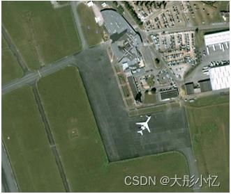
• 原图
  

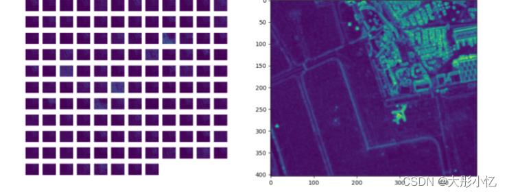
• conv1
  

• conv2
  

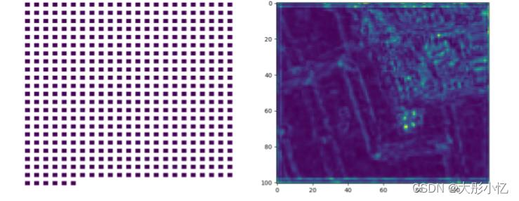
• conv3
  

• conv4
  

• conv5
  

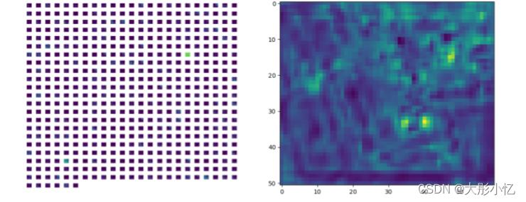
  通过分析上面的结果，可以发现浅层特征更多的是对图像边缘的检测，检测到的细节信息更多，随着层次的加深，特征图越来抽象，忽略了很多信息。

  参考文章：https://blog.csdn.net/Vici__/article/details/100626406
       https://blog.csdn.net/raby_gyl/article/details/79075716
       https://blog.csdn.net/mr_muli/article/details/90677623
       https://blog.csdn.net/missyougoon/article/details/85645195