AVOD:点云数据与BEV图的处理及可视化
Posted 夏小悠
tags:
篇首语:本文由小常识网(cha138.com)小编为大家整理,主要介绍了AVOD:点云数据与BEV图的处理及可视化相关的知识,希望对你有一定的参考价值。
文章目录
前言
本篇主要记录对AVOD代码的学习与理解,主要是KITTI数据集中3D Object Detection任务中的点云数据和BEV图的处理,为方面理解其中的操作,博主在这里加入了可视化的操作。
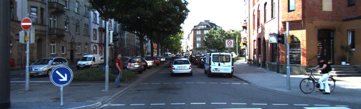
本篇博客使用的样本编号为
000274,RGB图像如下:
1. 点云数据可视化
点云数据保存在velodyne文件夹内,数据文件的格式是.bin,保存了x, y, z三轴坐标以及反射值r信息,数据格式为float32,通过numpy可以读取文件,具体如下:
import numpy as np


if __name__ == '__main__':
    bin_file = r'F:\\DataSet\\Kitti\\object\\velodyne\\000274.bin'
    pointcloud = np.fromfile(bin_file, dtype=np.float32, count=-1).reshape([-1, 4])
    print('pointcloud shape: ', pointcloud.shape)

# pointcloud shape:  (120438, 4)
为了更加直观的看点云图像,这里不再使用matplotlib,而是更专业的三维可视化工具包mayavi,具体操作如下:
import numpy as np
from mayavi import mlab


if __name__ == '__main__':
	bin_file = r'F:\\DataSet\\Kitti\\object\\velodyne\\000274.bin'
	pointcloud = np.fromfile(bin_file, dtype=np.float32, count=-1).reshape([-1, 4])

	x = pointcloud[:, 0]  # x position of point
	y = pointcloud[:, 1]  # y position of point
	z = pointcloud[:, 2]  # z position of point
	r = pointcloud[:, 3]  # reflectance value of point

	d = np.sqrt(x ** 2 + y ** 2)  # Map Distance from sensor

	vals = 'height'
	if vals == "height":
	    col = z
	else:
	    col = d

	fig = mlab.figure(bgcolor=(1, 1, 1), size=(700, 500))
	mlab.points3d(x, y, z,
	              d,  # Values used for Color
	              mode="point",
	              colormap='spectral',  # 'bone', 'copper', 'gnuplot', 'spectral', 'summer'
	              # color=(0, 1, 0),   # Used a fixed (r,g,b) instead
	              figure=fig)
	mlab.show()
可视化结果如下:
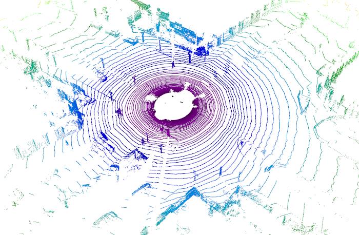
调整一下视角与RGB图保持一致:

2. 点云数据校准
RGB图片使用的是左侧第二个彩色摄像机,即image_2,因此需要将雷达数据进行坐标变化,将其映射到摄像机坐标系中,计算公式为:
y = P2 * R0_rect * Tr_velo_to_cam * x
大致计算流程:
# Read calibration info
frame_calib = calib_utils.read_calibration(calib_dir, img_idx)
x, y, z, i = calib_utils.read_lidar(velo_dir=velo_dir, img_idx=img_idx)

# Calculate the point cloud
pts = np.vstack((x, y, z)).T
pts = calib_utils.lidar_to_cam_frame(pts, frame_calib)

# Only keep points in front of camera (positive z)
pts = pts[pts[:, 2] > 0]
point_cloud = pts.T

# Project to image frame
point_in_im = calib_utils.project_to_image(point_cloud, p=frame_calib.p2).T
具体实现:
# 为了方便可视化数据,这里封装了对点云进行可视化的函数
def visu_point_cloud(x, y, z):
    d = np.sqrt(x ** 2 + y ** 2)  # Map Distance from sensor

    vals = 'distance'
    if vals == "distance":
        col = d
    else:
        col = z

    fig = mlab.figure(bgcolor=(1, 1, 1), size=(700, 500))
    mlab.points3d(x, y, z,
                  col,  # Values used for Color
                  mode="point",
                  colormap='spectral',  # 'bone', 'copper', 'gnuplot', 'spectral', 'summer'
                  # color=(0, 1, 0),   # Used a fixed (r,g,b) instead
                  figure=fig)

    mlab.show()


def get_lidar_point_cloud(calib_dir, velo_dir, img_idx, im_size=None, min_intensity=None):
    """ Calculates the lidar point cloud, and optionally returns only the
    points that are projected to the image.
    :param calib_dir: directory with calibration files
    :param velo_dir: directory with velodyne files
    :param img_idx: image index
    :param im_size: (optional) 2 x 1 list containing the size of the image
                      to filter the point cloud [w, h]
    :param min_intensity: (optional) minimum intensity required to keep a point
    :return: (3, N) point_cloud in the form [[x,...][y,...][z,...]]
    """

    # Read calibration info
    frame_calib = read_calibration(calib_dir, img_idx)
    x, y, z, i = read_lidar(velo_dir=velo_dir, img_idx=img_idx)

    # Calculate the point cloud
    pts = np.vstack((x, y, z)).T
    pts = lidar_to_cam_frame(pts, frame_calib)

    # The given image is assumed to be a 2D image
    if not im_size:
        point_cloud = pts.T
        return point_cloud

    else:
        # Only keep points in front of camera (positive z)
        pts = pts[pts[:, 2] > 0]
        point_cloud = pts.T

        # Project to image frame
        point_in_im = project_to_image(point_cloud, p=frame_calib['p2']).T

        # Filter based on the given image size
        image_filter = (point_in_im[:, 0] > 0) & \\
                       (point_in_im[:, 0] < im_size[0]) & \\
                       (point_in_im[:, 1] > 0) & \\
                       (point_in_im[:, 1] < im_size[1])

    if not min_intensity:
        return pts[image_filter].T

    else:
        intensity_filter = i > min_intensity
        point_filter = np.logical_and(image_filter, intensity_filter)
        return pts[point_filter].T


img_path = r'F:\\DataSet\\Kitti\\object\\image_2'
lidar_path = r'F:\\DataSet\\Kitti\\object\\velodyne'
calib_path = r'F:\\DataSet\\Kitti\\object\\calib'
planes_path = r'F:\\DataSet\\Kitti\\object\\planes'
label_path = r'F:\\DataSet\\Kitti\\object\\label_2'
img_idx = 274


if __name__ == '__main__':
    point_cloud = get_lidar_point_cloud(calib_path, lidar_path, img_idx, im_size)
    visu_point_cloud(point_cloud[0], point_cloud[1], point_cloud[2])
可视化结果如下:
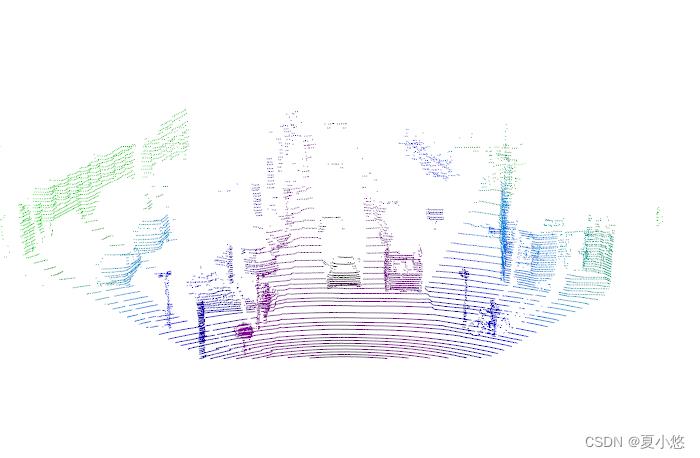
调整视角为俯视图:

3. 转为BEV图
BEV,即bird's eye view,鸟瞰图
鸟瞰图的计算需要用到地面数据,即空间上的点投影到某个平面,需要知道该平面的平面方程,平面方程的表达式为:
a
x
+
b
y
+
c
z
+
d
=
0
ax+by+cz+d=0
ax+by+cz+d=0 空间上的点
P
(
x
0
,
y
0
,
z
0
)
P(x_0,y_0,z_0)
P(x0,y0,z0)到平面上的距离为:
d
i
s
t
a
n
c
e
=
∣
a
x
0
+
b
y
0
+
c
z
0
+
d
∣
a
2
+
b
2
+
c
2
distance=\\frac |ax_0+by_0+cz_0+d| \\sqrt a^2+b^2+c^2
distance=a2+b2+c2∣ax0+by0+cz0+d∣ 读取KITTI数据集中的地面数据:
# 000274.txt
# Plane
Width 4
Height 1
-2.143976e-03 -9.997554e-01 2.201096e-02 1.707479e+00
# 分别表示a, b, c, d四个参数值
点云数据转BEV时高度分辨率为0.5,根据点云数据可以得到x,y和z轴上的数据,即x_col,y_col,z_col,然后使用np.lexsort()对x轴进行排序:
sorted_order = np.lexsort((y_col, z_col, x_col))
# 对 x_col 进行排序
# 如果 x_col 中的数值一样,则比较 z_col 中相应索引下的值的大小
# 如果还相同,再比较 y_col 中的元素
将 y_col 中的元素置为0,即只保留x和z轴上的数据,然后使用np.view()对数值类型进行变换:
# 定义12字节的数据类型
dt = np.dtype((np.void, 12))

# 先使用np.ascontiguousarray将一个内存不连续存储的数组转换为内存连续存储的数组,使得运行速度更快
# 再使用np.view按指定方式对内存区域进行切割,来完成数据类型的转换
# discrete_pts(n, 3) --> contiguous_array(n, 1)
# itemsize输出array元素的字节数
contiguous_array = np.ascontiguousarray(discrete_pts).view(dtype=dt)
离散点云数据discrete_pts的shape为(n,3),其数值类型为np.int32,4字节,总字节为n34Byte,现将其转为12Byte的数据,即保持总字节数不变:n112,转换完成后的shape为(n,1)。
对上述的数据进行去重:
# 去除数组中的重复数字,并进行排序
_, unique_indices = np.unique(contiguous_array, return_index=True)
unique_indices.sort()
# 得到不重复的数据
# voxel 体素(三维)
# pixel 像素(二维)
voxel_coords = discrete_pts[unique_indices]
# 将索引值映射到原点
voxel_coords -= -400
计算每个体素中数据点的数量,即后一个索引值减去当前索引值:
num_points_in_voxel = np.diff(unique_indices)
num_points_in_voxel = np.append(num_points_in_voxel,
                                discrete_pts_2d.shape[0] -
                                unique_indices[-1])
计算每个体素中数据点的高度,通过计算点到平面方程的距离:
# voxel (x, y, z)
# 平面方程: ax + by + cz + d = 0
height_in_voxel = (a*x + b*y + c*z + d) / np.sqrt(a**2 + b**2 + c**2)
对高度信息进行缩放,height_in_voxel = height_in_voxel / 0.5,根据二维索引值voxel_coords(去除y轴)与高度信息即可得到BEV数据,密度信息的计算:
# N is num points in voxel
# x = 16
density_map = min(1.0, log(N+1)/log(x))
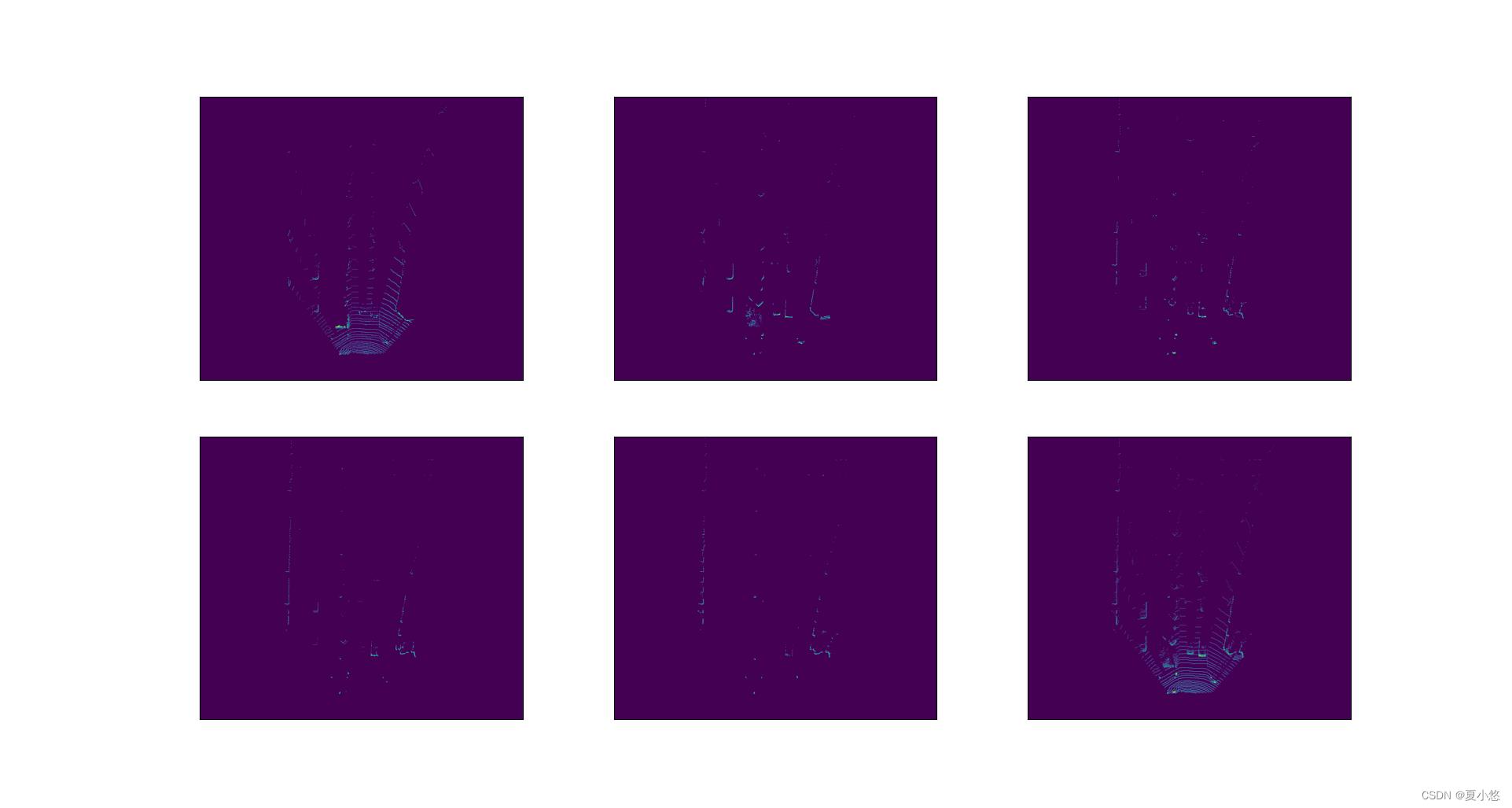
最终的BEV是由5个高度信息和1个密度信息组成,其shape为(700, 800, 6)。
三维可视化结果如下:

RGB可视化如下:
结束语
后续继续更新^_^
以上是关于AVOD:点云数据与BEV图的处理及可视化的主要内容,如果未能解决你的问题,请参考以下文章