LSTM实现环境质量预测的实现

Posted 2022-11-12 彭祥.

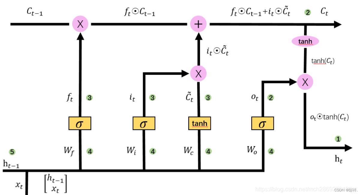
LSTM可以实现时序数据的预测，下面以一个环境质量变化的时序序列来介绍其实现和处理过程。

LSTM模型

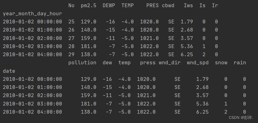
数据集介绍

首先是数据集：里面有9个变量值，其中包含时间和其他环境指标变量
，经过数据处理过程效果如下：

from pandas import read_csv
from datetime import datetime
# load data
def parse(x):
	return datetime.strptime(x, '%Y %m %d %H')
dataset = read_csv('raw.csv',  parse_dates = [['year', 'month', 'day', 'hour']], index_col=0, date_parser=parse)
print(dataset.head(5))
dataset.drop('No', axis=1, inplace=True)
# manually specify column names
dataset.columns = ['pollution', 'dew', 'temp', 'press', 'wnd_dir', 'wnd_spd', 'snow', 'rain']
dataset.index.name = 'date'
# mark all NA values with 0
dataset['pollution'].fillna(0, inplace=True)
# drop the first 24 hours
dataset = dataset[:]
# summarize first 5 rows
print(dataset.head(5))
# save to file
dataset.to_csv('pollution.csv')

主要是将原数据的日期格式进行规范，删除一些缺失值数据来生成我们需要的数据集。

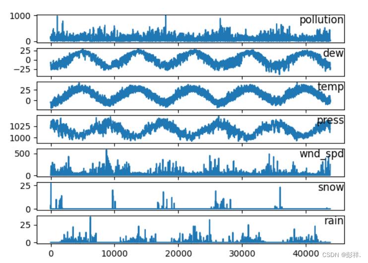
图表展示

将数据进行图表输出：

from pandas import read_csv
from matplotlib import pyplot
# load dataset
dataset = read_csv('pollution.csv', header=0, index_col=0)
values = dataset.values
# specify columns to plot
groups = [0, 1, 2, 3, 5, 6, 7]
i = 1
# plot each column
pyplot.figure()
for group in groups:
	pyplot.subplot(len(groups), 1, i)
	pyplot.plot(values[:, group])
	pyplot.title(dataset.columns[group], y=0.5, loc='right')
	i += 1
pyplot.show()

接下便是模型读取数据，训练，评估的过程了：
其实现的是一个多步长，多变量的时间序列预测过程：

生成监督数据

首先对数据集进行处理为监督数据，将其转换为3–>1的预测数据格式。

# 转换成监督数据，四列数据，3->1，三组预测一组
def series_to_supervised(data, n_in=1, n_out=1, dropnan=True):
    n_vars = 1 if type(data) is list else data.shape[1]
    df = DataFrame(data)
    cols, names = list(), list()
    # input sequence (t-n, ... t-1)
    # 将3组输入数据依次向下移动3，2，1行，将数据加入cols列表（技巧：(n_in, 0, -1)中的-1指倒序循环，步长为1）
    for i in range(n_in, 0, -1):
    	cols.append(df.shift(i))
    	names += [('var%d(t-%d)' % (j+1, i)) for j in range(n_vars)]
    # forecast sequence (t, t+1, ... t+n)
    # 将一组输出数据加入cols列表（技巧：其中i=0）
    for i in range(0, n_out):
    	cols.append(df.shift(-i))
    	if i == 0:
    		names += [('var%d(t)' % (j+1)) for j in range(n_vars)]
    	else:
    		names += [('var%d(t+%d)' % (j+1, i)) for j in range(n_vars)]
    # cols列表(list)中现在有四块经过下移后的数据(即：df(-3),df(-2),df(-1),df)，将四块数据按列 并排合并
    agg = concat(cols, axis=1)
    # 给合并后的数据添加列名
    agg.columns = names
    print(agg)
    # 删除NaN值列
    if dropnan:
    	agg.dropna(inplace=True)
    return agg

读取数据，并进行风向编码：将单词变为数据，并进行标准化缩放

# load dataset
dataset = read_csv('pollution.csv', header=0, index_col=0)
values = dataset.values
# 对“风向”列进行整数编码
encoder = LabelEncoder()
values[:,4] = encoder.fit_transform(values[:,4])#fit_transform就是将序列重新排列后再进行标准化
print(values[:,4])
values = values.astype('float32')
# 标准化/放缩 特征值在（0,1）之间
scaler = MinMaxScaler(feature_range=(0, 1))
scaled = scaler.fit_transform(values)

转换为监督数据：

# 用3小时数据预测一小时数据，8个特征值
n_hours = 3
n_features = 8
# 构造一个3->1的监督学习型数据
reframed = series_to_supervised(scaled, n_hours, 1)
print(reframed.shape)

所得的数据格式：(43797, 32)即有43797条数据，按每个小时划分，32个变量值

划分训练集与测试集，并设置输入值与输出值，设置前一年的数据进行训练，取每组数据的前38个为输入值，后18为输出值，取剩下的数据，即三年数据为测试集。

values = reframed.values
# 用一年的数据来训练
n_train_hours = 365 * 24
train = values[:n_train_hours, :]
test = values[n_train_hours:, :]
# split into input and outputs
n_obs = n_hours * n_features
# 有32=(4*8)列数据，取前24=(3*8) 列作为X，倒数第8列=(第25列)作为Y
train_X, train_y = train[:, :n_obs], train[:, -n_features]
test_X, test_y = test[:, :n_obs], test[:, -n_features]
print(train_X.shape, len(train_X), train_y.shape)

(8760, 24) 8760 (8760,)
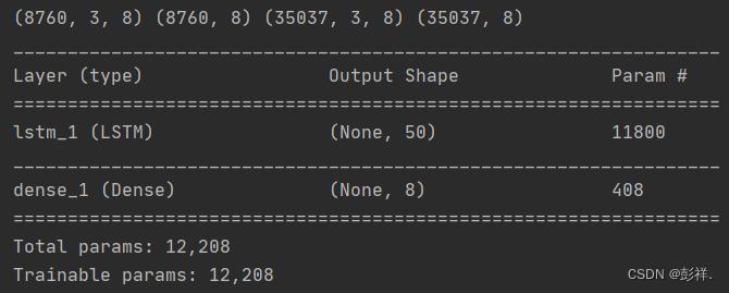
(8760, 3, 8) (8760,) (35037, 3, 8) (35037,)

设计网络模型

# 设计网络
model = Sequential()
model.add(LSTM(50, input_shape=(train_X.shape[1], train_X.shape[2])))
model.add(Dense(1))
model.compile(loss='mae', optimizer='adam')

拟合网络

history = model.fit(train_X, train_y, epochs=50, batch_size=8, validation_data=(test_X, test_y), verbose=2, shuffle=False)

图表展示数据误差值

# plot history
pyplot.plot(history.history['loss'], label='train')
pyplot.plot(history.history['val_loss'], label='test')
pyplot.legend()
pyplot.show()

数据预测

# 执行预测
yhat = model.predict(test_X)
# 将数据格式化成 n行 * 24列
test_X = test_X.reshape((test_X.shape[0], n_hours*n_features))
# 将预测列据和后7列数据拼接，因后续逆缩放时，数据形状要符合 n行*8列 的要求
inv_yhat = concatenate((yhat, test_X[:, -7:]), axis=1)
# 对拼接好的数据进行逆缩放
inv_yhat = scaler.inverse_transform(inv_yhat)
inv_yhat = inv_yhat[:,0]

test_y = test_y.reshape((len(test_y), 1))
# 将真实列据和后7列数据拼接，因后续逆缩放时，数据形状要符合 n行*8列 的要求
inv_y = concatenate((test_y, test_X[:, -7:]), axis=1)
# 对拼接好的数据进行逆缩放
inv_y = scaler.inverse_transform(inv_y)
inv_y = inv_y[:,0]

# 计算RMSE误差值
rmse = sqrt(mean_squared_error(inv_y, inv_yhat))
print('Test RMSE: %.3f' % rmse)

系统改进

之前博主在看这个系统时，发现了几个问题，即他最终的输出结果是pollution等级，他是如何实现的呢？
首先，在切分数据集是，他取前24列作为已知序列，使用倒数第8列为预测数列，即标签：

# 有32=(4*8)列数据，取前24=(3*8) 列作为X，倒数第8列=(第25列)作为Y
train_X, train_y = train[:, :n_obs], train[:, -n_features]#注意这里的-n_features是倒数第8列而非倒数最后8列
test_X, test_y = test[:, :n_obs], test[:, -n_features]

确定了我们的输出结果为1列，那么我们最后的全连接层设为1即可：

model = Sequential()
model.add(LSTM(50, input_shape=(train_X.shape[1], train_X.shape[2])))
model.add(Dense(1))

然后我们的数据格式如何规范呢，在我们的fit这里就做了限定：

history = model.fit(train_X, train_y, epochs=2, batch_size=8, validation_data=(test_X, test_y), verbose=2, shuffle=False)#指明了训练集测试集，这也叫声明了格式

那么到这里问题就很清晰了，如果我想让我的结果为八个属性值呢，我们只需要这样做：将标签取后8个：

# 有32=(4*8)列数据，取前24=(3*8) 列作为X，倒数后8列=(第25列)作为Y
train_X, train_y = train[:, :n_obs], train[:, -n_features:]
test_X, test_y = test[:, :n_obs], test[:, -n_features:]
print(train_X.shape, len(train_X), train_y.shape,train_y)
# 将数据转换为3D输入，timesteps=3，3条数据预测1条 [samples, timesteps, features]
train_X = train_X.reshape((train_X.shape[0], n_hours, n_features))
test_X = test_X.reshape((test_X.shape[0], n_hours, n_features))
train_Y = train_y.reshape((train_y.shape[0], 1, n_features))
test_Y = test_y.reshape((test_y.shape[0], 1, n_features))
#并进行格式转换

对网络的输出结果进行限定，全连接层改为8

model = Sequential()
model.add(LSTM(50,input_shape=(train_X.shape[1], train_X.shape[2])))
model.add(Dense(8))

其余不用改变，这样他的输出结果变为后8个变量了