AndrewNg机器学习编程作业python实现及心得总结
Posted MichaelIp
tags:
篇首语:本文由小常识网(cha138.com)小编为大家整理,主要介绍了AndrewNg机器学习编程作业python实现及心得总结相关的知识,希望对你有一定的参考价值。
作业目录
- 作业一(Week2 ex1)
- 作业二(Week3 ex2)
- 作业三(Week4 ex3)
- 作业四(Week5 ex4)
- 作业五(Week6 ex5)
- 作业六(Week7 ex6)
- 作业七(Week8 ex7)
- 作业八(Week9 ex8)
作业结构:
作业一(Week2 ex1)
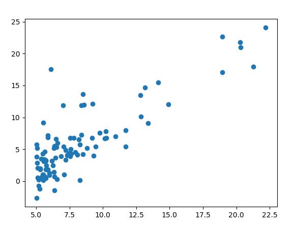
在本部分的练习中,您将使用一个变量实现线性回归,以预测食品卡车的利润。假设你是一家餐馆的首席执行官,正在考虑不同的城市开设一个新的分店。该连锁店已经在各个城市拥有卡车,而且你有来自城市的利润和人口数据。
您希望使用这些数据来帮助您选择将哪个城市扩展到下一个城市。
ex1data1.txt 是本次作业数据,我们打印出来如图:
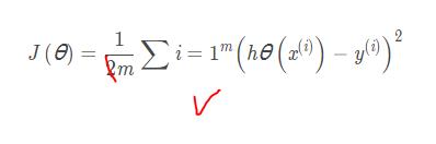
线性回归的代价函数:
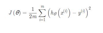
其中1/2m的1/2只是方便求导,求梯度(平方的导数是乘以2, 刚好和1/2约了),网上也有些公式是没有1/2的, 都是正确的, 不影响后面的分析。
权重优化公式

红线部分为梯度公式, 也就是代价函数的导数。
α 是学习率, 之所以之前1/2可以约去, 是因为1/2只是个常数, 后面可以用α 来兜底, 来控制梯度的大小。
下面用python实现本周编程作业:
ex1必做题:
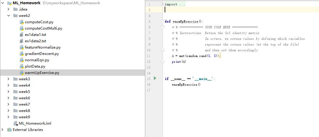
warmUpExercise.py:
from numpy import *;

def warmUpExercise():
    # % ============= YOUR CODE HERE ==============
    # % Instructions: Return the 5x5 identity matrix
    # %               In octave, we return values by defining which variables
    # %               represent the return values (at the top of the file)
    # %               and then set them accordingly.
    A = mat(random.rand(5, 5));
    print(A)

if __name__ == '__main__':
    warmUpExercise()
computeCost.py:
from numpy import *;
import numpy as np;
import math;
import pandas as pd
import matplotlib.pyplot as plt

def computeCost(X, y, theta):
    #COMPUTECOST Compute cost for linear regression
    #   J = COMPUTECOST(X, y, theta) computes the cost of using theta as the
    #   parameter for linear regression to fit the data points in X and y
    #
    # Initialize some useful values
    m = len(y); # number of training examples
    # You need to return the following variables correctly
    J = 0;
    # ====================== YOUR CODE HERE ======================
    # Instructions: Compute the cost of a particular choice of theta
    #               You should set J to the cost.
    J = np.sum( np.power((X.dot(theta.T)-y),2) )/(2 * m)
    # =========================================================================
    return J

if __name__ == '__main__':
    path = 'ex1data1.txt'
    data = pd.read_csv(path, header=None)
    X = np.matrix(data[0])
    y = np.matrix(data[1])
    m = X.shape[1]
    X = X.reshape(m,1)
    y = y.reshape(m,1)
    theta = np.zeros((1,1))
    print('X.shape',X.shape)
    print('theta.shape',theta.shape)
    print('y.shape',y.shape)
    J = computeCost(X, y, theta)
    print('J',J)
输出:
X.shape (97, 1)
theta.shape (1, 1)
y.shape (97, 1)
J 32.072733877455676
gradientDescent.py:
from numpy import *;
from computeCost import computeCost
import numpy as np;
import math;
import pandas as pd
import matplotlib.pyplot as plt
from plotData import plotData
def gradientDescent(X, y, theta, alpha, num_iters):
#GRADIENTDESCENT Performs gradient descent to learn theta
# theta = GRADIENTDESCENT(X, y, theta, alpha, num_iters) updates theta by
# taking num_iters gradient steps with learning rate alpha
# Initialize some useful values
m = X.shape[0] # number of training examples
J_history = np.zeros(num_iters);
for iter in range(num_iters):
# ====================== YOUR CODE HERE ======================
# theta.
#
# Hint: While debugging, it can be useful to print out the values
# of the cost function (computeCost) and gradient here.
#
theta = theta - alpha/m * (( X.dot(theta.T) - y ).T.dot(X))
J = computeCost(X, y, theta)
J_history[iter] = J
return theta, J_history
if __name__ == '__main__':
path = 'ex1data1.txt'
data = pd.read_csv(path, header=None)
cols = data.shape[1]
X = data.iloc[:,0:cols-1]
y = data.iloc[:,cols-1:cols]
X = np.matrix(X.values)
y = np.matrix(y.values)
theta = np.zeros((1,1))
alpha = 0.001
epoch = 20
theta, J_history = gradientDescent(X, y, theta, alpha, epoch)
print('theta',theta)
print('J_history',J_history)
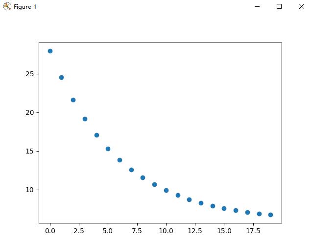
plotData(np.arange(0,epoch,1), J_history)
输出:
theta [[0.65565076]]
J_history [27.97858553 24.52386652 21.60870997 19.1488463  17.07316731 15.32167052
 13.84372475 12.59660645 11.54426468 10.656279    9.90698007  9.2747076
  8.74118426  8.29098728  7.91110265  7.59054888  7.32005961  7.0918157
  6.89921922  6.73670271]
选择题:
featureNormalize.py:
from numpy import *;
import numpy as np;
import math;
import pandas as pd
import matplotlib.pyplot as plt

def featureNormalize(X):
    #FEATURENORMALIZE Normalizes the features in X
    #   FEATURENORMALIZE(X) returns a normalized version of X where
    #   the mean value of each feature is 0 and the standard deviation
    #   is 1. This is often a good preprocessing step to do when
    #   working with learning algorithms.

    # You need to set these values correctly

    # ====================== YOUR CODE HERE ======================
    # Instructions: First, for each feature dimension, compute the mean
    #               of the feature and subtract it from the dataset,
    #               storing the mean value in mu. Next, compute the
    #               standard deviation of each feature and divide
    #               each feature by it's standard deviation, storing
    #               the standard deviation in sigma.
    #
    #               Note that X is a matrix where each column is a
    #               feature and each row is an example. You need
    #               to perform the normalization separately for
    #               each feature.
    #
    # Hint: You might find the 'mean' and 'std' functions useful.
    #
    mu = X.mean()
    sigma = X.std()
    X_norm = (X - mu)/sigma
    return X_norm, mu, sigma

if __name__ == '__main__':
    path = 'ex1data2.txt'
    data = pd.read_csv(path, header=None)
    cols = data.shape[1]  # 列数
    X = data.iloc[:,0:cols-1]  # 取前cols-1列,即输入向量
    y = data.iloc[:,cols-1:cols] # 取最后一列,即目标向量
    X = np.matrix(X.values)
    y = np.matrix(y.values)
    theta = np.zeros((1,2))
    X_norm, mu, sigma = featureNormalize(X)
    # print('X_norm',X_norm)
    print('mu',mu)
    print('sigma',sigma)
输出:
mu 1001.9255319148937
sigma 1143.0528202028345
computeCostMulti.py:
from numpy import *;
import numpy as np;
import math;
import pandas as pd
import matplotlib.pyplot as plt

path = 'ex1data2.txt'
data = pd.read_csv(path, header=None)
cols = data.shape[1]  # 列数
X = data.iloc[:,0:cols-1]  # 取前cols-1列,即输入向量
y = data.iloc[:,cols-1:cols] # 取最后一列,即目标向量
X = np.matrix(X.values)
y = np.matrix(y.values)
theta = np.matrix([0,0])

def computeCostMulti(X, y, theta):
    #COMPUTECOSTMULTI Compute cost for linear regression with multiple variables
    #   J = COMPUTECOSTMULTI(X, y, theta) computes the cost of using theta as the
    #   parameter for linear regression to fit the data points in X and y

    # Initialize some useful values
    m = len(y); # number of training examples

    # You need to return the following variables correctly
    J = 0;

    # ====================== YOUR CODE HERE ======================
    # Instructions: Compute the cost of a particular choice of theta
    #               You should set J to the cost.

    J = np.sum( np.power((X*theta.T-y),2) )/(2 * m)

    # # =========================================================================
    return J

if __name__ == '__main__':
    print(X.shape)
    print(theta.shape)
    print(y.shape)
    J = computeCostMulti(X, y, theta)
    print(J)
输出:
(47, 2)
(1, 2)
(47, 1)
65591548106.45744
normalEqn.py:
from numpy import *;
import numpy as np;
import math;
import pandas as pd
import matplotlib.pyplot as plt

def normalEqn(X, y):
    #NORMALEQN Computes the closed-form solution to linear regression
    #   NORMALEQN(X,y) computes the closed-form solution to linear
    #   regression using the normal equations.


    # ====================== YOUR CODE HERE ======================
    # Instructions: Complete the code to compute the closed form solution
    #               to linear regression and put the result in theta.
    #

    # ---------------------- Sample Solution ----------------------

    theta = np.linalg.inv(X.T * X) * X.T * y

    # -------------------------------------------------------------
    # ============================================================
    return theta


if __name__ == '__main__':
    path = 'ex1data2.txt'
    data = pd.read_csv(path, header=None)
    cols = data.shape[1]  # 列数
    X = data.iloc[:,0:cols-1]  # 取前cols-1列,即输入向量
    y = data.iloc[:,cols-1:cols] # 取最后一列,即目标向量
    X = np.matrix(X.values)
    y = np.matrix(y.values)
    theta = np.matrix([0,0])
    theta = normalEqn(X, y)
    print('theta',theta)
输出:
theta [[  140.86108621]
 [16978.19105903]]
作业二(Week3 ex2)
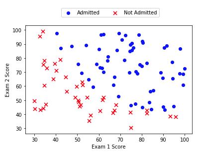
在这部分的练习中,你将建立一个逻辑回归模型来预测一个学生是否能进入大学。假设你是一所大学的行政管理人员,你想根据两门考试的结果,来决定每个申请人是否被录取。你有以前申请人的历史数据,可以将其用作逻辑回归训练集。对于每一个训练样本,你有申请人两次测评的分数以及录取的结果。为了完成这个预测任务,我们准备构建一个可以基于两次测试评分来评估录取可能性的分类模型。
下图是ex2data1.txt数据模型图:
逻辑回归的假设函数:

其中的 g代表逻辑回归的S形函数(Sigmoid function):
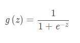
大概长这样:
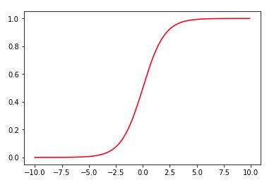
y值在0到1之间,大于等于0.5归一类,小于0.5归一类。
逻辑回归的代价函数:
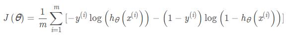
和线性回归的代价函数略有不同, 看似复杂,其实原理差不多。
下面用python实现本周编程作业:
sigmoid.py:
from numpy import *;
import numpy as np;
import math;
import pandas as pd
import matplotlib.pyplot as plt

def sigmoid(z):
    #SIGMOID Compute sigmoid function
    #   g = SIGMOID(z) computes the sigmoid of z.

    # You need to return the following variables correctly
    # g = zeros(size(z));

    # ====================== YOUR CODE HERE ======================
    # Instructions: Compute the sigmoid of each value of z (z can be a matrix,
    #               vector or scalar).

    g = 1 / ( 1 + np.exp(-z))

    # =============================================================
    return g


if __name__ == '__main__':
    x1 = np.arange(-10, 10, 0.1)
    g = sigmoid(x1)
    plt.plot(x1, sigmoid(x1), c='r')
    plt.show()
输出:

costFunction.py:
from numpy import *;
import numpy as np;
import math;
import pandas as pd
from sigmoid import sigmoid
import matplotlib.pyplot as plt

def costFunction(theta, X, y):
    #COSTFUNCTION Compute cost and gradient for logistic regression
    #   J = COSTFUNCTION(theta, X, y) computes the cost of using theta as the
    #   parameter for logistic regression and the gradient of the cost
    #   w.r.t. to the parameters.

    # Initialize some useful values
    m = len(y); # number of training examples

    # You need to return the following variables correctly
    # J = 0;
    # grad = zeros(size(theta));

    # ====================== YOUR CODE HERE ======================
    # Instructions: Compute the cost of a particular choice of theta.
    #               You should set J to the cost.
    #               Compute the partial derivatives and set grad to the partial
    #               derivatives of the cost w.r.t. each parameter in theta
    #
    # Note: grad should have the same dimensions as theta
    #
    h = sigmoid(X.dot(theta.T))
    J = 1/m * np.sum(-np.multiply(y,np.log(h)) - np.multiply((1-y),np.log(1-h)))
    grad = (h -y).T * X/m
    # =============================================================
    return J, grad


if __name__ == '__main__':
    path = 'ex2data1.txt'
    data = pd.read_csv(path, header=None)
    cols = data.shape[1]  # 列数
    X = data.iloc[:,0:cols-1]  # 取前cols-1列,即输入向量
    y = data.iloc[:,cols-1:cols] # 取最后一列,即目标向量
    X = np.matrix(X.values)
    y = np.matrix(y.values)
    theta = np.matrix([0,0])
    # print('X.shape',X.shape)
    # print('theta.shape',theta.shape)
    # print('y.shape',y.shape)
    J, grad = costFunction(theta, X, y)
    print('J',J)
    print('grad',grad)
输出:
J 0.6931471805599453
grad [[-12.00921659 -11.26284221]]
costFunctionReg.py:
from numpy import *;
import numpy as np;
import math;
import pandas as pd
import costFunction as cf
import sigmoid as s
import matplotlib.pyplot as plt

def costFunctionReg(theta, X, y, lamb_da):
    #COSTFUNCTIONREG Compute cost and gradient for logistic regression with regularization
    #   J = COSTFUNCTIONREG(theta, X, y, lambda) computes the cost of using
    #   theta as the parameter for regularized logistic regression and the
    #   gradient of the cost w.r.t. to the parameters.

    # Initialize some useful values
    m = len(y); # number of training examples

    # You need to return the following variables correctly
    # J = 0;
    # grad = zeros(size(theta));

    # ====================== YOUR CODE HERE ======================
    # Instructions: Compute the cost of a particular choice of theta.
    #               You should set J to the cost.
    #               Compute the partial derivatives and set grad to the partial
    #               derivatives of the cost w.r.t. each parameter in theta
    J, grad= cf.costFunction(theta, X, y)
    theta = theta[: 1]
    J += lamb_da/2*m*(theta * theta.T)
    grad += lamb_da/m*theta

    # =============================================================
    return J, grad


if __name__ == '__main__':

    path = 'ex2data2.txt'
    data = pd.read_csv(path, header=None)
    cols = data.shape[1]  # 列数
    X = data.iloc[:,0:cols-1]  # 取前cols-1列,即输入向量
    y = data.iloc[:,cols-1:cols] # 取最后一列,即目标向量
    X = np.matrix(X.values)
    y = np.matrix(y.values)
    theta = np.matrix([0,0])
    # print('X.shape',X.shape)
    # print('theta.shape',theta.shape)
    # print('y.shape',y.shape)
    J, grad = costFunctionReg(theta, X, y, lamb_da=1)
    print('J',J)
    print('grad',grad)
输出:
J [[0.69314718]]
grad [[1.87880932e-02 7.77711864e-05]]
predict.py:
from numpy import *;
import numpy as np;
import math;
import pandas as pd
import sigmoid as s
import costFunction as cf
import matplotlib.pyplot as plt
import scipy.optimize as opt

path = 'ex2data2.txt'
data = pd.read_csv(path, header=None)
cols = data.shape[1]  # 列数
X = data.iloc[:,0:cols-1]  # 取前cols-1列,即输入向量
y = data.iloc[:,cols-1:cols] # 取最后一列,即目标向量
X = np.matrix(X.values)
y = np.matrix(y.values)
theta = np.matrix([0.20623159,   0.20147149])

def predict(theta, X):
    #PREDICT Predict whether the label is 0 or 1 using learned logistic
    #regression parameters theta
    #   p = PREDICT(theta, X) computes the predictions for X using a
    #   threshold at 0.5 (i.e., if sigmoid(theta'*x) >= 0.5, predict 1)

    m = X.shape[0]; # Number of training examples

    # You need to return the following variables correctly
    # p = zeros(m, 1);

    # ====================== YOUR CODE HERE ======================
    # Instructions: Complete the following code to make predictions using
    #               your learned logistic regression parameters.
    #               You should set p to a vector of 0's and 1's
    #
    h = s.sigmoid(X*theta.T)
    # p = np.matrix(data.iloc[:,cols-1:cols].values)
    # for i in range(m):
    #     if h[i][0]>=0.5:
    #         p[i][0] = 1
    #     else:
    #         p[i][0] = 0
    p = [1 if x >= 0.5 else 0 for x in h]
    # =========================================================================
    return p

if __name__ == '__main__':
    print(X.shape)
    print(theta.shape)
    print(y.shape)
    p = predict(theta, X)
    print(p)
输出:
(118, 2)
(1, 2)
(118, 1)
[1, 1, 1, 1, 0, 0, 0, 0, 0, 0, 0, 1, 1, 1, 1, 1, 1, 1, 1, 1, 0, 0, 0, 0, 0, 0, 0, 1, 1, 1, 1, 1, 1, 1, 0, 0, 0, 0, 0, 0, 1, 1, 1, 1, 1, 1, 1, 1, 1, 1, 1, 1, 1, 1, 0, 0, 0, 0, 1, 1, 1, 1, 1, 1, 1, 1, 1, 1, 1, 1, 1, 1, 1, 1, 0, 0, 1, 0, 0, 0, 0, 0, 0, 0, 0, 0, 0, 0, 1, 1, 1, 1, 1, 1, 1, 1, 1, 1, 1, 1, 1, 1, 0, 0, 0, 0, 0, 0, 0, 0, 0, 0, 0, 0, 0, 1, 1, 1]
作业三(Week4 ex3)
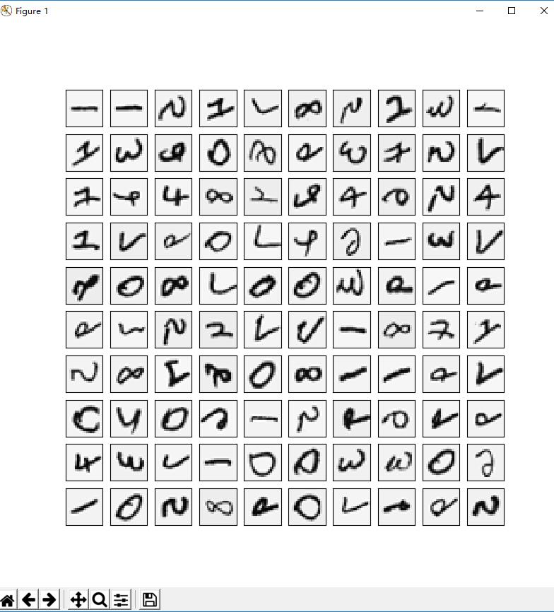
我们将扩展我们在练习2中写的logistic回归的实现,并将其应用于一对多的分类(不止两个类别)。
下面用plot_100_image方法根据ex3data1.mat随机画100个数字:
def plot_100_image(X):
    sample_idx = np.random.choice(np.arange(X.shape[0]), 100)  # 随机选100个样本
    sample_images = X[sample_idx, :]  # (100,400)

    fig, ax_array = plt.subplots(nrows=10, ncols=10, sharey=True, sharex=True, figsize=(8, 8))

    for row in range(10):
        for column in range(10):
            ax_array[row, column].matshow(sample_images[10 * row + column].reshape((20, 20)),
                                          cmap='gray_r')
    plt.xticks([])
    plt.yticks([])
    plt.show()
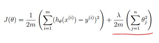
正则化的logistic回归的代价函数:

红色部分就是正则化部分, 前面就是之前提到的逻辑回归代价函数公式。
下面用python实现本周编程作业:
lrCostFunction.py:
import numpy as np
import pandas as pd
import matplotlib.pyplot as plt
from scipy.io import loadmat

def lrCostFunction(theta, X, y, lamb_da):
    # LRCOSTFUNCTION Compute cost and gradient for logistic regression with
    # regularization
    #   J = LRCOSTFUNCTION(theta, X, y, lambda) computes the cost of using
    #   theta as the parameter for regularized logistic regression and the
    #   gradient of the cost w.r.t. to the parameters.

    # Initialize some useful values
    m = len(y);  # number of training examples

    # You need to return the following variables correctly
    # J = 0;
    # grad = zeros(size(theta));

    # ====================== YOUR CODE HERE ======================
    # Instructions: Compute the cost of a particular choice of theta.
    #               You should set J to the cost.
    #               Compute the partial derivatives and set grad to the partial
    #               derivatives of the cost w.r.t. each parameter in theta
    #
    # Hint: The computation of the cost function and gradients can be
    #       efficiently vectorized. For example, consider the computation
    #
    #           sigmoid(X * theta)
    #
    #       Each row of the resulting matrix will contain the value of the
    #       prediction for that example. You can make use of this to vectorize
    #       the cost function and gradient computations.
    #
    # Hint: When computing the gradient of the regularized cost function,
    #       there're many possible vectorized solutions, but one solution
    #       looks like:
    #           grad = (unregularized gradient for logistic regression)
    #           temp = theta;
    #           temp(1) = 0;   # because we don't add anything for j = 0
    #           grad = grad + YOUR_CODE_HERE (using the temp variable)

    J = compute_J(theta, X, y, lamb_da, m)
    grad = compute_grad(theta, X, y, lamb_da, m)

    # =============================================================
    return J, grad


def compute_J(theta, X, y, lamb_da, m):
    y = y.reshape(y.size,1)
    theta = theta.reshape(1,theta.size)
    h = sigmoid(X.dot(theta.T))
    # theta = theta[:,1:]
    theta[0] = 1
    J = 1 / m * np.sum(-np.multiply(y, np.log(h)) - np.multiply((1 - y), np.log(1 - h))) + lamb_da / (2 * m) * (
        theta.dot(theta.T))
    # J = 1 / m * np.sum(-np.multiply(y, np.log(h)) - np.multiply((1 - y), np.log(1 - h)))
    return J


def compute_grad(theta, X, y, lamb_da, m):
    y = y.reshape(y.size,1)
    theta = theta.reshape(1,theta.size)
    h = sigmoid(X.dot(theta.T))
    # theta = theta[:,1:]
    theta[0] = 1
    grad = 1 / m * X.T.dot(h - y) + (lamb_da / m) * theta.T
    # grad = 1 / m * X.T.dot(h - y)
    return grad


def sigmoid(z):
    g = 1 / (1 + np.exp(-z));
    return g


def load_data(path):
    data = loadmat(path)
    X = data['X']
    y = data['y']
    return X, y


if __name__ == '__main__':
    X, y = load_data('ex3data1.mat')
    theta = np.zeros((1, X.shape[1]))
    J, grad = lrCostFunction(theta, X, y, lamb_da=1)
    print('J.shape',J.shape)
    print('J',J)
    print('grad.shape',grad.shape)
输出:
J.shape (1, 1)
J [[160.43425758]]
grad.shape (400, 1)
oneVsAll.py:
import numpy as np
import pandas as pd
import matplotlib.pyplot as plt
from scipy.io import loadmat
from scipy.optimize import minimize

from lrCostFunction import compute_J, compute_grad, sigmoid,load_data

def oneVsAll(X, y, num_labels, lamb_da):
    # ONEVSALL trains multiple logistic regression classifiers and returns all
    # the classifiers in a matrix all_theta, where the i-th row of all_theta
    # corresponds to the classifier for label i
    #   [all_theta] = ONEVSALL(X, y, num_labels, lambda) trains num_labels
    #   logistic regression classifiers and returns each of these classifiers
    #   in a matrix all_theta, where the i-th row of all_theta corresponds
    #   to the classifier for label i

    # Some useful variables
    m, n = X.shape

    # You need to return the following variables correctly
    all_theta = np.zeros((num_labels, n))

    # Add ones to the X data matrix
    # X = [ones(m, 1) X];

    # ====================== YOUR CODE HERE ======================
    # Instructions: You should complete the following code to train num_labels
    #               logistic regression classifiers with regularization
    #               parameter lambda.
    #
    # Hint: theta(:) will return a column vector.
    #
    # Hint: You can use y == c to obtain a vector of 1's and 0's that tell you
    #       whether the ground truth is true/false for this class.
    #
    # Note: For this assignment, we recommend using fmincg to optimize the cost
    #       function. It is okay to use a for-loop (for c = 1:num_labels) to
    #       loop over the different classes.
    #
    #       fmincg works similarly to fminunc, but is more efficient when we
    #       are dealing with large number of parameters.
    #
    # Example Code for fmincg:
    #
    #     # Set Initial theta
    #     initial_theta = zeros(n + 1, 1);
    #
    #     # Set options for fminunc
    #     options = optimset('GradObj', 'on', 'MaxIter', 50);
    #
    #     # Run fmincg to obtain the optimal theta
    #     # This function will return theta and the cost
    #     [theta] = ...
    #         fmincg (@(t)(lrCostFunction(t, X, (y == c), lambda)), ...
    #                 initial_theta, options);

    for i in range(1, num_labels + 1):
        theta = np.zeros((1, X.shape[1]))
        y_i = np.array([1 if label == i else 0 for label in y])
        ret = minimize(fun=compute_J, x0=theta, args=(X, y_i, lamb_da, m), method='TNC',
                       jac=compute_grad, options='disp': True)
        all_theta[i - 1, :] = ret.x

    # =========================================================================
    return all_theta


if __name__ == '__main__':
    X, y = load_data('ex3data1.mat')
    all_theta = oneVsAll(X, y, num_labels=10, lamb_da=1)
    print(all_theta.shape)
输出:
(10, 400)
predict.py:
import numpy as np
import pandas as pd
import matplotlib.pyplot as plt
from scipy.io import loadmat
from scipy.optimize import minimize

from lrCostFunction import compute_J, compute_grad, sigmoid,load_data
from oneVsAll import oneVsAll

def predict(Theta1, Theta2, X):
    #PREDICT Predict the label of an input given a trained neural network
    #   p = PREDICT(Theta1, Theta2, X) outputs the predicted label of X given the
    #   trained weights of a neural network (Theta1, Theta2)

    # Useful values
    m = X.shape[0]

    # You need to return the following variables correctly
    # p = zeros(size(X, 1), 1);

    # ====================== YOUR CODE HERE ======================
    # Instructions: Complete the following code to make predictions using
    #               your learned neural network. You should set p to a
    #               vector containing labels between 1 to num_labels.
    #
    # Hint: The max function might come in useful. In particular, the max
    #       function can also return the index of the max element, for more
    #       information see 'help max'. If your examples are in rows, then, you
    #       can use max(A, [], 2) to obtain the max for each row.

    # Add ones to the X data matrix  -jin

    a2 = sigmoid(X.dot(Theta1.T))
    a2 = np.insert(a2, 0, values=np.ones(a2.shape[0]), axis=1)
    a3 = sigmoid(a2.dot(Theta2.T))
    p = np.argmax(a3, axis=1) + 1
    p = p.reshape(p.size,1)
    # =========================================================================
    return p

def load_weight(path):
    data = loadmat(path)
    return data['Theta1'], data['Theta2']

if __name__ == '__main__':
    theta1, theta2 = load_weight('ex3weights.mat')
    X, y = load_data('ex3data1.mat')
    X = np.insert(X, 0, values=np.ones(X.shape[0]), axis=1)
    p = predict(theta1, theta2, X)
    accuracy = np.mean(p == y)
    print ('accuracy = 0%'.format(accuracy * 100))
输出:
accuracy = 97.52%
predictOneVsAll.py:
import numpy as np
import pandas as pd
import matplotlib.pyplot as plt
from scipy.io import loadmat
from scipy.optimize import minimize

from lrCostFunction import compute_J, compute_grad, sigmoid,load_data
from oneVsAll import oneVsAll

def predictOneVsAll(all_theta, X):
    #PREDICT Predict the label for a trained one-vs-all classifier. The labels
    #are in the range 1..K, where K = size(all_theta, 1).
    #  p = PREDICTONEVSALL(all_theta, X) will return a vector of predictions
    #  for each example in the matrix X. Note that X contains the examples in
    #  rows. all_theta is a matrix where the i-th row is a trained logistic
    #  regression theta vector for the i-th class. You should set p to a vector
    #  of values from 1..K (e.g., p = [1; 3; 1; 2] predicts classes 1, 3, 1, 2
    #  for 4 examples)

    m = X.shape[0]
    num_labels = all_theta.shape[0]

    # You need to return the following variables correctly
    # p = zeros(size(X, 1), 1);

    # Add ones to the X data matrix
    # X = [ones(m, 1) X];

    # ====================== YOUR CODE HERE ======================
    # Instructions: Complete the following code to make predictions using
    #               your learned logistic regression parameters (one-vs-all).
    #               You should set p to a vector of predictions (from 1 to
    #               num_labels).
    #
    # Hint: This code can be done all vectorized using the max function.
    #       In particular, the max function can also return the index of the
    #       max element, for more information see 'help max'. If your examples
    #       are in rows, then, you can use max(A, [], 2) to obtain the max
    #       for each row.

    p = sigmoid(X.dot(all_theta.T))
    p = np.argmax(p, axis=1)
    p = p + 1

    # =========================================================================
    return p


if __name__ == '__main__':
    X, y = load_data('ex3data1.mat')
    all_theta = oneVsAll( X, y, num_labels=10,  lamb_da=1)
    y_pred = predictOneVsAll(all_theta,X)
    y_pred = y_pred.reshape(y_pred.size,1)
    accuracy = np.mean(y_pred == y)
    print ('accuracy = 0%'.format(accuracy * 100))
输出:
accuracy = 97.39999999999999%
作业四(Week5 ex4)
这周被称作“绝望第五周”,需要实现反向传播算法来学习神经网络的参数。依旧是上次预测手写数数字的例子。
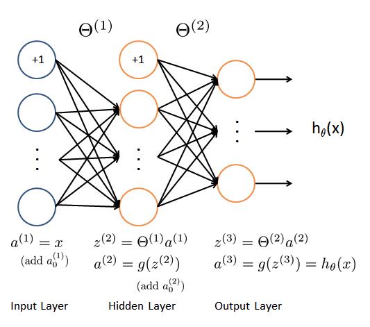
正向传递过程,其中 g 为sigmoid激活函数:

反向传播过程:
先算误差:
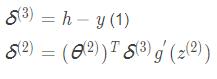
再算梯度:
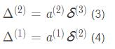
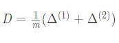
最后网络的总梯度为:
这里的反向传播有点绕,我另一篇文章有详细手写推导过程:
【用高中的知识点徒手推导逻辑回归中的反向梯队】
下面用python实现本周编程作业:
sigmoidGradient.py:
import numpy as np
import pandas as pd
import matplotlib.pyplot as plt
from scipy.io import loadmat

def sigmoidGradient(z):
    # SIGMOIDGRADIENT returns the gradient of the sigmoid function
    # evaluated at z
    #   g = SIGMOIDGRADIENT(z) computes the gradient of the sigmoid function
    #   evaluated at z. This should work regardless if z is a matrix or a
    #   vector. In particular, if z is a vector or matrix, you should return
    #   the gradient for each element.

    # g = zeros(size(z));

    # ====================== YOUR CODE HERE ======================
    # Instructions: Compute the gradient of the sigmoid function evaluated at
    #               each value of z (z can be a matrix, vector or scalar).
    h = sigmoid(z)
    g = np.multiply(h, (1 - h))

    # =============================================================
    return g


def sigmoid(z):
    g = 1 / (1 + np.exp(-z));
    return g


def load_data(path):
    data = loadmat(path)
    X = data['X']
    y = data['y']
    return X, y

def load_weight(path):
    data = loadmat(path)
    return data['Theta1'], data['Theta2']

if __name__ == '__main__':
    X, y = load_data('ex4data1.mat')
    theta = np.zeros((1, X.shape[1]))
    z = np.dot(X, theta.T)
    g = sigmoidGradient(z)
    print('g', g)
输出:
g [[0.25]
[0.25]
[0.25]
...
[0.25]
[0.25]
[0.25]]
nnCostFunction.py:
import numpy as np
import pandas as pd
import matplotlib.pyplot as plt
from scipy.io import loadmat
from sigmoidGradient import sigmoid, load_data, load_weight, sigmoidGradient

def nnCostFunction(nn_params, input_layer_size, hidden_layer_size, num_labels, X, y, lamb_da):
    # NNCOSTFUNCTION Implements the neural network cost function for a two layer
    # neural network which performs classification
    #   [J grad] = NNCOSTFUNCTON(nn_params, hidden_layer_size, num_labels, ...
    #   X, y, lambda) computes the cost and gradient of the neural network. The
    #   parameters for the neural network are "unrolled" into the vector
    #   nn_params and need to be converted back into the weight matrices.
    #
    #   The returned parameter grad should be a "unrolled" vector of the
    #   partial derivatives of the neural network.
    #

    # Reshape nn_params back into the parameters Theta1 and Theta2, the weight matrices
    # for our 2 layer neural network
    # Theta1 = reshape(nn_params(1:hidden_layer_size * (input_layer_size + 1)), ...
    # hidden_layer_size, (input_layer_size + 1));
    #
    # Theta2 = reshape(nn_params((1 + (hidden_layer_size * (input_layer_size + 1))):end), ...
    # num_labels, (hidden_layer_size + 1));
    # Theta1 = np.zeros(hidden_layer_size,input_layer_size+1)
    # Theta2 = np.zeros(num_labels,hidden_layer_size+1)

    # Setup some useful variables
    m = X.shape[0]

    # You need to return the following variables correctly
    J = 0;
    # Theta1_grad = zeros(size(Theta1));
    # Theta2_grad = zeros(size(Theta2));

    # ====================== YOUR CODE HERE ======================
    # Instructions: You should complete the code by working through the
    #               following parts.
    #
    # Part 1: Feedforward the neural network and return the cost in the
    #         variable J. After implementing Part 1, you can verify that your
    #         cost function computation is correct by verifying the cost
    #         computed in ex4.m
    #
    # Part 2: Implement the backpropagation algorithm to compute the gradients
    #         Theta1_grad and Theta2_grad. You should return the partial derivatives of
    #         the cost function with respect to Theta1 and Theta2 in Theta1_grad and
    #         Theta2_grad, respectively. After implementing Part 2, you can check
    #         that your implementation is correct by running checkNNGradients
    #
    #         Note: The vector y passed into the function is a vector of labels
    #               containing values from 1..K. You need to map this vector into a
    #               binary vector of 1's and 0's to be used with the neural network
    #               cost function.
    #
    #         Hint: We recommend implementing backpropagation using a for-loop
    #               over the training examples if you are implementing it for the
    #               first time.
    #
    # Part 3: Implement regularization with the cost function and gradients.
    #
    #         Hint: You can implement this around the code for
    #               backpropagation. That is, you can compute the gradients for
    #               the regularization separately and then add them to Theta1_grad
    #               and Theta2_grad from Part 2.
    #
    Theta1, Theta2 = load_weight('ex4weights.mat')

    # Part 1
    X = np.insert(X, 0, values=np.ones(X.shape[0]), axis=1)
    a2 = sigmoid(X.dot(Theta1.T))
    a2 = np.insert(a2, 0, values=np.ones(a2.shape[0]), axis=1)
    a3 = sigmoid(a2.dot(Theta2.T))

    cy = np.zeros((m, num_labels))
    for i in range(m):
        cy[i, y[i] - 1] = 1

    Theta1 = Theta1[:, 1:]
    Theta2 = Theta2[:, 1:]

    J = compute_J(Theta1, Theta2, a3, m, cy, lamb_da)

    grad = compute_grad(a2,a3, Theta2, cy, m)

    # =========================================================================
    return J, grad


def compute_J(Theta1, Theta2, a3, m, cy, lamb_da):
    J = 1 / m * np.sum(-np.multiply(cy, np.log(a3)) - np.multiply((1 - cy), np.log(1 - a3)))

    th1 = 0
    th2 = 0
    for i in range(Theta1.shape[0]):
        t_tmp = Theta1[i, :]
        th1 += np.sum(t_tmp.dot(t_tmp.T))
    for i in range(Theta2.shape[0]):
        t_tmp = Theta2[i, :]
        th2 += np.sum(t_tmp.dot(t_tmp.T))

    J += lamb_da / (2 * m) * (th1 + th2)
    return J
def compute_grad(a2,a3, Theta2, cy, m):
    delta3 = a3 - cy  # (5000,10)
    delta2 = np.multiply(delta3.dot(Theta2), sigmoidGradient(a2[:,1:]))  # (5000,25)
    Theta1_grad = delta2.T.dot(X)  # (25,401)
    Theta2_grad = delta3.T.dot(a2)  # (10,26)
    t1_t2 = np.r_[Theta1_grad.flatten(), Theta2_grad.flatten()]  # np.r_是按列连接两个矩阵,就是把两矩阵上下相加,要求列数相等。
    grad = (1 / m) * t1_t2  # (10285,)
    return grad

if __name__ == '__main__':
    X, y = load_data('ex4data1.mat')
    J, grad = nnCostFunction(nn_params=1, input_layer_size=10, hidden_layer_size=25, num_labels=10, X=X, y=y, lamb_da=1)
    print('J', J)
    print('grad.shape', grad.shape)
输出:
J 0.38376985909092365
grad.shape (10260,)
作业五(Week6 ex5)
在前半部分的练习中,你将实现正则化线性回归,以预测水库中的水位变化,从而预测大坝流出的水量。在下半部分中,您将通过一些调试学习算法的诊断,并检查偏差 v.s. 方差的影响。
根据ex5data1.mat打印出这次数据的模样:
线性回归正则化代价函数:
和逻辑回归正则化代价函数一样, 前面都是正儿八经的线性回归代价函数 , 红色部分就是正则化函数。
线性回归正则化梯度:

下面用python实现本周编程作业:
learningCurve.py:
import numpy as np
import pandas as pd
import matplotlib.pyplot as plt
from scipy.io import loadmat
import scipy.optimize as opt
from linearRegCostFunction import compute_grad, compute_J, linearRegCostFunction

def learningCurve(X, y, Xval, yval, lamb_da):
   #LEARNINGCURVE Generates the train and cross validation set errors needed
   #to plot a learning curve
   #   [error_train, error_val] = ...
   #       LEARNINGCURVE(X, y, Xval, yval, lambda) returns the train and
   #       cross validation set errors for a learning curve. In particular,
   #       it returns two vectors of the same length - error_train and
   #       error_val. Then, error_train(i) contains the training error for
   #       i examples (and similarly for error_val(i)).
   #
   #   In this function, you will compute the train and test errors for
   #   dataset sizes from 1 up to m. In practice, when working with larger
   #   datasets, you might want to do this in larger intervals.
   #

   # Number of training examples
   m = X.shape[0]

   # You need to return these values correctly
   # error_train = np.zeros((m, 1))
   # error_val   = np.zeros((m, 1))
   error_train, error_val = [], []

   # ====================== YOUR CODE HERE ======================
   # Instructions: Fill in this function to return training errors in
   #               error_train and the cross validation errors in error_val.
   #               i.e., error_train(i) and
   #               error_val(i) should give you the errors
   #               obtained after training on i examples.
   #
   # Note: You should evaluate the training error on the first i training
   #       examples (i.e., X(1:i, :) and y(1:i)).
   #
   #       For the cross-validation error, you should instead evaluate on
   #       the _entire_ cross validation set (Xval and yval).
   #
   # Note: If you are using your cost function (linearRegCostFunction)
   #       to compute the training and cross validation error, you should
   #       call the function with the lambda argument set to 0.
   #       Do note that you will still need to use lambda when running
   #       the training to obtain the theta parameters.
   #
   # Hint: You can loop over the examples with the following:
   #
   #       for i = 1:m
   #           # Compute train/cross validation errors using training examples
   #           # X(1:i, :) and y(1:i), storing the result in
   #           # error_train(i) and error_val(i)
   #           ....
   #
   #       end
   #

   # ---------------------- Sample Solution ----------------------

   for i in range(1, m+1):
       theta = trainLinearReg(X[:i], y[:i], lamb_da)
       error_train.append(compute_J(theta, X[:i], y[:i], lamb_da, m))
       error_val.append(compute_J(theta,  Xval, yval, lamb_da, m))

   # -------------------------------------------------------------

   # =========================================================================
   return error_train, error_val

def trainLinearReg(X, y, l):
   theta = np.zeros(X.shape[1])
   m = len(X)
   res = opt.minimize(fun=compute_J,
                      x0=theta,
                      args=(X, y, l, m),
                      method='TNC',
                      jac=compute_grad)
   return res.x

if __name__ == '__main__':
   data = loadmat('ex5data1.mat')
   X, y = data['X'], data['y']
   Xval, yval = data['Xval'], data['yval']
   X = np.insert(X, 0, 1, axis=1)
   Xval = np.insert(Xval, 0, 1, axis=1)
   theta = np.zeros((1, X.shape[1]))
   error_train, error_val = learningCurve(X, y, Xval, yval,0)
   print('error_train', error_train)
   print('error_val', error_val)
输出:
error_train [array([[0.18980339]]), array([[0.24715886]]), array([[49.43667484]]), array([[105.97979737]]), array([[106.30855924]]), array([[106.49601542]]), array([[115.51234849]]), array([[115.79709682]]), array([[116.379967]]), array([[116.960197]]), array([[119.38441281]]), array([[140.95412088]])]
error_val [array([[287.20263926]]), array([[287.20263926]]), array([[287.20263926]]), array([[287.20263926]]), array([[287.20263926]]), array([[287.20263926]]), array([[287.20263926]]), array([[287.20263926]]), array([[287.20263926]]), array([[287.20263926]]), array([[287.20263926]]), array([[287.20263926]])]
linearRegCostFunction.py:
import numpy as np
import pandas as pd
import matplotlib.pyplot as plt
from scipy.io import loadmat

def linearRegCostFunction(X, y, theta, lamb_da):
    # LINEARREGCOSTFUNCTION Compute cost and gradient for regularized linear
    # regression with multiple variables
    #   [J, grad] = LINEARREGCOSTFUNCTION(X, y, theta, lambda) computes the
    #   cost of using theta as the parameter for linear regression to fit the
    #   data points in X and y. Returns the cost in J and the gradient in grad

    # Initialize some useful values
    m = len(y);  # number of training examples

    # You need to return the following variables correctly
    # J = 0;
    # grad = zeros(size(theta));

    # ====================== YOUR CODE HERE ======================
    # Instructions: Compute the cost and gradient of regularized linear
    #               regression for a particular choice of theta.
    #
    #               You should set J to the cost and grad to the gradient.
    #

    J = compute_J(theta, X, y, lamb_da, m)
    grad = compute_grad(theta, X, y, lamb_da, m)

    # =========================================================================
    return J, grad


def compute_J(theta, X, y, lamb_da, m):
    y = y.reshape(y.size, 1)
    theta = theta.reshape(1, theta.size)
    h = X.dot(theta.T)
    # theta = theta[:,1:]
    theta[0] = 0
    J = (1 / (2 * m)) * np.sum(np.square(h - y)) + lamb_da / (2 * m) * (theta.dot(theta.T))
    return J


def compute_grad(theta, X, y, lamb_da, m):
    y = y.reshape(y.size, 1)
    theta = theta.reshape(1, theta.size)
    h = X.dot(theta.T)
    # theta = theta[:,1:]
    # grad = 1 / m * (h - y).T.dot(X) + np.concatenate((np.zeros((1, 1)), (lamb_da / m) * theta))
    theta[0] = 0
    grad = 1 / m * (h - y).T.dot(X) + (lamb_da / m) * theta
    return grad


if __name__ == '__main__':
    data = loadmat('ex5data1.mat')
    X, y = data['X'], data['y']
    X = np.insert(X, 0, 1, axis=1)
    theta = np.ones((1, X.shape[1]))
    J, grad = linearRegCostFunction(X, y, theta, lamb_da=1)
    print('X=,y='.format(X.shape, y.shape))
    print('theta='.format(theta.shape))
    print('J', J)
    print('grad.shape', grad.shape)
    print('grad', grad)
输出:
X=(12, 2),y=(12, 1)
theta=(1, 2)
J [[303.95152555]]
grad.shape (1, 2)
grad [[ -11.21758933 -245.65199649]]
polyFeatures.py:
import numpy as np
import pandas as pd
import matplotlib.pyplot as plt
from scipy.io import loadmat
import scipy.optimize as opt
from linearRegCostFunction import compute_grad,compute_J, linearRegCostFunction


def polyFeatures(X, p):
    #POLYFEATURES Maps X (1D vector) into the p-th power
    #   [X_poly] = POLYFEATURES(X, p) takes a data matrix X (size m x 1) and
    #   maps each example into its polynomial features where
    #   X_poly(i, :) = [X(i) X(i).^2 X(i).^3 ...  X(i).^p];
    #


    # You need to return the following variables correctly.
    # X_poly = []
    X_poly = np.ones((len(X), p))

    # ====================== YOUR CODE HERE ======================
    # Instructions: Given a vector X, return a matrix X_poly where the p-th
    #               column of X contains the values of X to the p-th power.
    #
    #
    for i in range(1, p):
        X_poly[:,i] = np.power(X, i).flatten()
    # =========================================================================
    return X_poly

if __name__ == '__main__':
    data = loadmat('ex5data1.mat')
    X, y = data['X'], data['y']
    X_poly = polyFeatures(X, 6)
    print('X_poly',X_poly)
输出:
X_poly [[ 1.00000000e+00 -1.59367581e+01  2.53980260e+02 -4.04762197e+03
  6.45059724e+04 -1.02801608e+06]
[ 1.00000000e+00 -2.91529792e+01  8.49896197e+02 -2.47770062e+04
  7.22323546e+05 -2.10578833e+07]
[ 1.00000000e+00  3.61895486e+01  1.30968343e+03  4.73968522e+04
  1.71527069e+06  6.20748719e+07]
[ 1.00000000e+00  3.74921873e+01  1.40566411e+03  5.27014222e+04
  1.97589159e+06  7.40804977e+07]
[ 1.00000000e+00 -4.80588295e+01  2.30965109e+03 -1.10999128e+05
  5.33448815e+06 -2.56369256e+08]
[ 1.00000000e+00 -8.94145794e+00  7.99496701e+01 -7.14866612e+02
  6.39194974e+03 -5.71533498e+04]
[ 1.00000000e+00  1.53077929e+01  2.34328523e+02  3.58705250e+03
  5.49098568e+04  8.40548715e+05]
[ 1.00000000e+00 -3.47062658e+01  1.20452489e+03 -4.18045609e+04
  1.45088020e+06 -5.03546340e+07]
[ 1.00000000e+00  1.38915437e+00  1.92974986e+00  2.68072045e+00
  3.72393452e+00  5.17311991e+00]
[ 1.00000000e+00 -4.43837599e+01  1.96991814e+03 -8.74323736e+04
  3.88057747e+06 -1.72234619e+08]
[ 1.00000000e+00  7.01350208e+00  4.91892115e+01  3.44988637e+02
  2.41957852e+03  1.69697190e+04]
[ 1.00000000e+00  2.27627489e+01  5.18142738e+02  1.17943531e+04
  2.68471897e+05  6.11115839e+06]]
validationCurve.py:
import numpy as np
import pandas as pd
import matplotlib.pyplot as plt
from scipy.io import loadmat
import scipy.optimize as opt
from linearRegCostFunction import compute_grad, compute_J, linearRegCostFunction


def validationCurve(X, y, Xval, yval):
   # VALIDATIONCURVE Generate the train and validation errors needed to
   # plot a validation curve that we can use to select lambda
   #   [lambda_vec, error_train, error_val] = ...
   #       VALIDATIONCURVE(X, y, Xval, yval) returns the train
   #       and validation errors (in error_train, error_val)
   #       for different values of lambda. You are given the training set (X,
   #       y) and validation set (Xval, yval).
   #

   # Selected values of lambda (you should not change this)
   lambda_vec = np.array([0, 0.001, 0.003, 0.01, 0.03, 0.1, 0.3, 1, 3, 10]).T

   # You need to return these variables correctly.
   # error_train = np.zeros((len(lambda_vec), 1))
   # error_val = np.zeros((len(lambda_vec), 1))
   error_train, error_val = [], []

   # ====================== YOUR CODE HERE ======================
   # Instructions: Fill in this function to return training errors in
   #               error_train and the validation errors in error_val. The
   #               vector lambda_vec contains the different lambda parameters
   #               to use for each calculation of the errors, i.e,
   #               error_train(i), and error_val(i) should give
   #               you the errors obtained after training with
   #               lambda = lambda_vec(i)
   #
   # Note: You can loop over lambda_vec with the following:
   #
   #       for i = 1:length(lambda_vec)
   #           lambda = lambda_vec(i);
   #           # Compute train / val errors when training linear
   #           # regression with regularization parameter lambda
   #           # You should store the result in error_train(i)
   #           # and error_val(i)
   #           ....
   #
   #       end
   #
   #

   m = len(lambda_vec)
   for i in range(m):
       lamb_da = lambda_vec[i]
       theta = trainLinearReg(X, y, lamb_da, m)
       error_train.append(linearRegCostFunction(X, y, theta, 0))
       error_val.append(linearRegCostFunction(Xval, yval, theta, 0))

   # =========================================================================
   return lambda_vec, error_train, error_val


def trainLinearReg(X, y, l, m):
   theta = np.zeros(X.shape[1])
   res = opt.minimize(fun=compute_J,
                      x0=theta,
                      args=(X, y, l, m),
                      method='TNC',
                      jac=compute_grad)
   return res.x


if __name__ == '__main__':
   data = loadmat('ex5data1.mat')
   X, y = data['X'], data['y']
   Xval, yval = data['Xval'], data['yval']
   X = np.insert(X, 0, 1, axis=1)
   Xval = np.insert(Xval, 0, 1, axis=1)
   theta = np.以上是关于AndrewNg机器学习编程作业python实现及心得总结的主要内容,如果未能解决你的问题,请参考以下文章