情感分析入门demo《Real-World Natural Language Processing》 chap2:Your first NLP application
Posted 临风而眠
tags:
篇首语:本文由小常识网(cha138.com)小编为大家整理,主要介绍了情感分析入门demo《Real-World Natural Language Processing》 chap2:Your first NLP application相关的知识,希望对你有一定的参考价值。
情感分析入门demo《Real-World Natural Language Processing》 chap2:Your first NLP application
书名为《Real-World Natural Language Processing》,由于chap2是本书的入门章节,所以很多基础概念像dataset,neural network这里依旧会介绍,不过之前在其他笔记里面记过了,下面遇到这些部分就尝试用自己的语言来概括复习
- This chapter covers
- Building a sentiment analyzer using AllenNLP
- Applying basic machine learning concepts (datasets, classification, and regression)
- Employing neural network concepts (word embeddings, recurrent neural networks, linear layers)
- Training the model through reducing loss
- Evaluating and deploying your model
- 本章的引言
- We are going to discuss how to do NLP in a more principled, modern way. Specifically, we’d like to build a sentiment analyzer using a neural network. Even though the sentiment analyzer we are going to build is a simple application and the library (AllenNLP) takes care of most heavy lifting(大多数繁重的工作), it is a full-fledged(成熟的,充分发展的) NLP application that covers a lot of basic components of modern NLP and machine learning. I’ll introduce important terms and concepts along the way.
2.1 Introducing sentiment analysis
-
sentiment analysis
- a technique used in the automatic identification and categorization of subjective information within text
- widely used in quantifying opinions, emotions and so on that are written in an unstructured way
- applied to a wide variety of textual resources such as survey, reviews, and social media
-
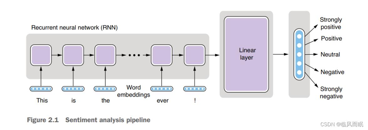
sentiment analysis pipeline
-
based on the supervised machine learning paradigm
- the system is trained on data that contains the desired labels for each input sentence
-
one of the most basic tasks in sentiment analysis is the classification of polarity, that is, to classify whether the expressed opinion is positive, negative,neutral, negative or strongly negative
- multiclass classification
2.2 Working with NLP datasets
2.2.1 What is a dataset?
关注几个概念
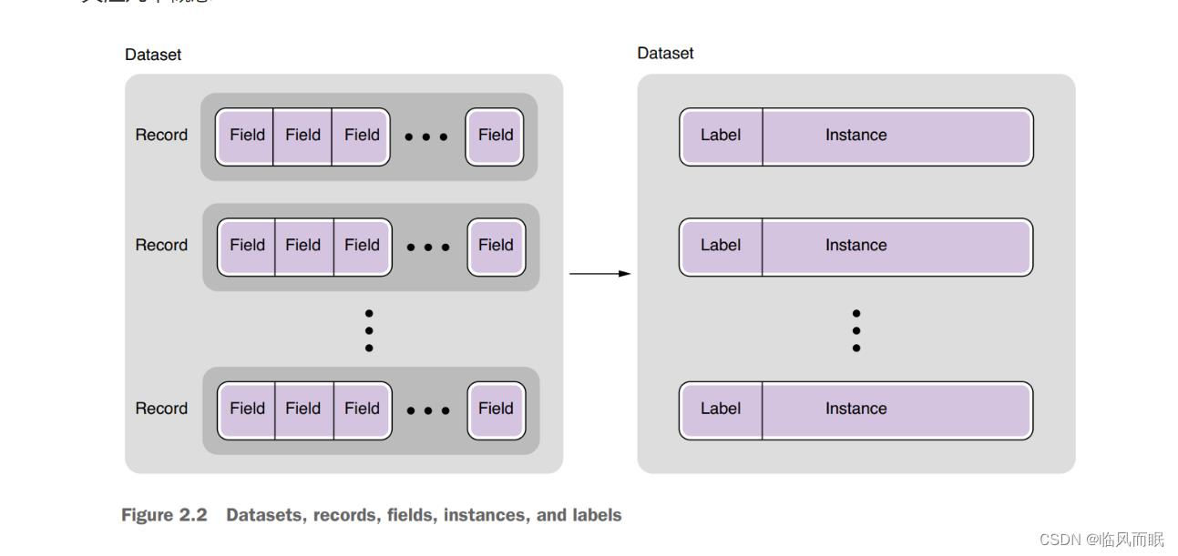
- In NLP, records in a dataset are usually some type of linguistic units, such as words, sentences, or documents.
- A dataset of natural language texts is called a corpus (plural: corpora).
- Some NLP datasets and corpora have more complex structures. For example, a dataset may contain a collection of sentences, where each sentence is annotated with detailed linguistic information, such as part-of-speech tags, parse trees, dependency structures, and semantic roles. If a dataset contains a collection of sentences annotated with their parse trees, the dataset is called a treebank. The most famous example of this is Penn Treebank (PTB).
- In machine learning, an instance is a basic unit for which the prediction is made.
- An instance is usually created from a record in a dataset
- this is not always the case—for example, if you take a treebank and use it to train an NLP task that detects all nouns in a sentence, then each word, not a sentence, becomes an instance, because prediction (noun or not noun) is made for each word.
- A label is a piece of information attached to some linguistic unit in a dataset.
2.2.2 Stanford Sentiment Treebank
-
这个是我们要用的数据集:Stanford Sentiment Treebank (SST; https://nlp.stanford.edu/sentiment/), one of the most widely used sentiment analysis datasets as of today.
-
some excerpts from the dataset
(4
 (2 (2 Steven) (2 Spielberg))
 (4
 (2 (2 brings) (3 us))
 (4 (2 another) (4 masterpiece))))
(1
 (2 It)
 (1
 (1 (2 (2 's) (1 not))
 (4 (2 a) (4 (4 great) (2 (2 monster) (2 movie)))))
 (2 .)))
-
-
One feature that differentiates SST from other datasets is the fact that sentiment labels are assigned not only to sentences but also to every word and phrase in sentences
- Each sentence is annotated with sentiment labels (4 and 1).
- Each word is also annotated, for example, (4 masterpiece) and (1 not).
- Every single phrase is also annotated, for example, (4 (2 another) (4 masterpiece)).
-
This property of the dataset enables us to study the complex semantic interactions between words and phrases. For example, let’s consider the polarity of the following sentence as a whole:
The movie was actually neither that funny, nor super witty.
-
The above statement would definitely be a negative, although, if you focus on the individual words (such as funny, witty), you might be fooled into thinking it’s a positive. If you built a simple classifier that takes “votes” from individual words (e.g., the sentence is positive if a majority of its words are positive), such classifiers would have difficulties classifying this example correctly. To correctly classify the polarity of this sentence, you need to understand the semantic impact of the negation “neither . . . nor.” For this property, SST has been used as the standard benchmark for neural network models that can capture the syntactic structures of sentences (www.realworldnlpbook.com/ch2.html#socher13).
-
However, in this chapter, we are going to ignore all the labels assigned to internal phrases and use only labels for sentences
这章只关心整个句子的情感标签
-
2.2.3 Train, validation, and test sets
-
In NLP and ML, it is common to use a couple of different types of datasets to develop and evaluate models. A widely used best practice is to use three different types of dataset splits—train, validation, and test sets
- A train (or training) set is the main dataset used to train the NLP/ML models.
- A validation set (also called a dev or development set) is used for model selection.
- the validation set gives a proxy for the model’s generalizability, 可以有效防止overfitting
- The validation set is also used for tuning hyperparameters.
- In fact, you can think of models with different hyperparameters as separate models, even if they have the same structure, and hyperparameter tuning can be considered one type of model selection.
- A test set is used to evaluate the model using a new, unseen set of data.
- you shouldn’t rely solely on a train set and a validation set to measure the generalizability of your model, because your model could also overfit to the validation set in a subtle way.
-
In summary, when training NLP models, use a train set to train your model candidates, use a validation set to choose good ones, and use a test set to evaluate them. Many public datasets used for NLP and ML evaluation are already split into train/ validation/test sets. If you just have a single dataset, you can split it into those three datasets by yourself. An 80:10:10 split is commonly used.
-
下图很清晰 depicts the train/ validation/test split as well as the entire training pipeline.

2.2.4 Loading SST datasets using AllenNLP
AllenNLP does not officially support Windows.
这里很棒,给出了colab的链接
-
首先安装必要的包,克隆仓库
!pip install allennlp==2.5.0
!pip install allennlp-models==2.5.0
!git clone https://github.com/mhagiwara/realworldnlp.git
%cd realworldnlp
感觉在colab里面 git clone 确实比上传文件要快
-
导入necessary classes and modules
from itertools import chain from typing import Dict import numpy as np import torch import torch.optim as optim from allennlp.data.data_loaders import MultiProcessDataLoader from allennlp.data.samplers import BucketBatchSampler from allennlp.data.vocabulary import Vocabulary from allennlp.models import Model from allennlp.modules.seq2vec_encoders import Seq2VecEncoder, PytorchSeq2VecWrapper from allennlp.modules.text_field_embedders import TextFieldEmbedder, BasicTextFieldEmbedder from allennlp.modules.token_embedders import Embedding from allennlp.nn.util import get_text_field_mask from allennlp.training import GradientDescentTrainer from allennlp.training.metrics import CategoricalAccuracy, F1Measure from allennlp_models.classification.dataset_readers.stanford_sentiment_tree_bank import \\ StanfordSentimentTreeBankDatasetReader from realworldnlp.predictors import SentenceClassifierPredictor -
设置两个constant
EMBEDDING_DIM = 128 HIDDEN_DIM = 128 -
AllenNLP already supports an abstraction called DatasetReader, which takes care of reading a dataset from the original format (be it raw text or some exotic XML-based format) and returns it as a collection of instances. We are going to use Stanford-SentimentTreeBankDatasetReader(), which is a type of DatasetReader that specifically deals with SST datasets, as shown here:
reader = StanfordSentimentTreeBankDatasetReader()
train_path = 'https://s3.amazonaws.com/realworldnlpbook/data/stanfordSentimentTreebank/trees/train.txt'
dev_path = 'https://s3.amazonaws.com/realworldnlpbook/data/stanfordSentimentTreebank/trees/dev.txt'
This snippet will create a dataset reader for SST datasets and define the paths for the train and dev text files.
2.3 Using word embeddings
From this section on, we’ll start building the neural network architecture for the sentiment analyzer. Architecture is just another word for the structure of neural networks. Building neural networks is a lot like building structures such as houses. The first step is to figure out how to feed the input (e.g., sentences for sentiment analysis) into the network.
As we have seen previously, everything in NLP is discrete, meaning there is no predictable relationship between the forms and the meanings (remember “rat” and “sat”). On the other hand, neural networks are best at dealing with something numerical and continuous, meaning everything in neural networks needs to be float numbers. How can we “bridge” between these two worlds—discrete and continuous? The key is the use of word embeddings, which we are going to discuss in detail in this section.
2.3.1 What are word embeddings?
-
Word embeddings are one of the most important concepts in modern NLP.
-
Technically, an **embedding ** a continuous vector representation of something that is usually discrete. A word embedding is a continuous vector representation of a word.
-
In simpler terms, word embeddings are a way to represent each word with a 300-element array (or an array of any other size) filled with nonzero float numbers. It is conceptually very simple.
-
Then, why has it been so important and prevalent in modern NLP? The history of NLP is actually the history of continuous battle against “discreteness” of language. In the eyes of computers, “cat” is no closer to “dog” than it is to “pizza.”
这句话意思是 When computers process language, they do not have the same understanding of the relationships between words as humans do. For example, humans know that a cat is a type of animal and that it is closely related to other animals such as dogs, while pizza is a food and is not related to animals at all. However, computers process language based on mathematical algorithms and do not have the same intuitive understanding of the relationships between words.
-
One way to deal with discrete words programmatically is to assign indices to individual words as follows (here we simply assume that these indices are assigned alphabetically)
index("cat") = 1
index("dog") = 2
index("pizza") = 3
…
These assignments are usually managed by a lookup table. The entire, finite set of words that one NLP application or task deals with is called vocabulary. But this method isn’t any better than dealing with raw words. Just because words are now represented by numbers doesn’t mean you can do arithmetic operations on them and conclude that “cat” is equally similar to “dog” (difference between 1 and 2), as “dog” is to “pizza” (difference between 2 and 3). Those indices are still discrete and arbitrary.
-
“What if we can represent them on a numerical scale?” some NLP researchers wondered decades ago. Can we think of some sort of numerical scale where words are represented as points, so that semantically closer words (e.g., “dog” and “cat,” which are both animals) are also geometrically closer?
This is a step forward.
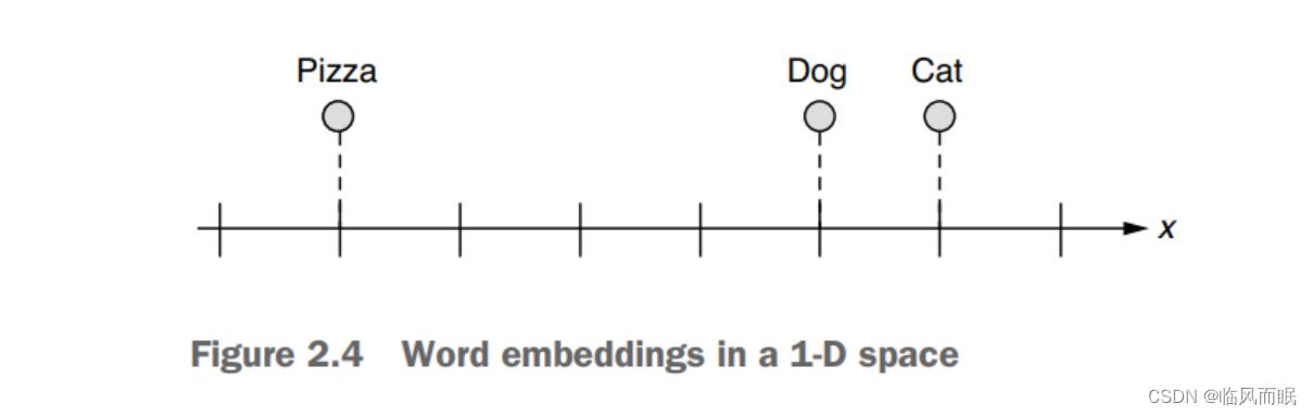
Now we can represent the fact that “cat” and “dog” are more similar to each other than “pizza” is to those words. But still, “pizza” is slightly closer to “dog” than it is to “cat.” What if you wanted to place it somewhere that is equally far from “cat” and “dog?” Maybe only one dimension is too limiting.
-
How about adding another dimension to this?
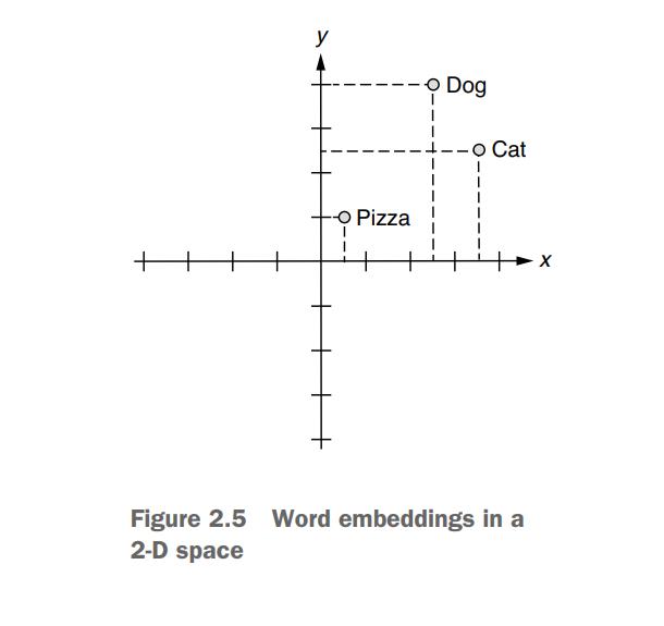
Much better! Because computers are really good at dealing with multidimensional spaces (because you can just represent points by arrays), you can simply keep doing this until you have a sufficient number of dimensions.Let’s have three dimensions. In this 3-D space, you can represent those three words as follows:
vec("cat") = [0.7, 0.5, 0.1]vec("dog") = [0.8, 0.3, 0.1]vec("pizza") = [0.1, 0.2, 0.8]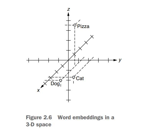
- The x -axis (the first element) here represents some concept of “animal-ness” and the z-axis (the third dimension) corresponds to “food-ness.” (I’m making these numbers up, but you get the point.) This is essentially what word embeddings are. You just embedded those words in a three-dimensional space. By using those vectors, you already “know” how the basic building blocks of the language work. For example, if you wanted to identify animal names, then you would just look at the first element of each word vector and see if the value is high enough. This is a great jump start compared to the raw word indices!
-
By the way, we have a much simpler method to “embed” words into a multidimensional space. Think of a multidimensional space that has as many dimensions as there are words. Then, give to each word a vector that is filled with zeros but just one 1, as shown next:
vec("cat") = [1, 0, 0]vec("dog") = [0, 1, 0]vec("pizza") = [0, 0, 1]Notice that each vector has only one 1 at the position corresponding to the word’s index. These special vectors are called one-hot vectors.
These vectors are not very useful themselves in representing semantic relationship between those words—the three words are all at the equal distance from each other—but they are still (a very dumb kind of) embeddings. They are often used as the input to a machine learning algorithm when embeddings are not available.
2.3.2 Using word embeddings for sentiment analysis
-
First, we create dataset loaders that take care of loading data and passing it to the training pipeline, as shown next:
sampler = BucketBatchSampler(batch_size=32, sorting_keys=["tokens"])
train_data_loader = MultiProcessDataLoader(reader, train_path, batch_sampler=sampler)
dev_data_loader = MultiProcessDataLoader(reader, dev_path, batch_sampler=sampler)
-
AllenNLP provides a useful
Vocabularyclass that manages mappings from some linguistic units (such as characters, words, and labels) to their IDs. You can tell the class to create aVocabularyinstance from a set of instances as follows:# You can optionally specify the minimum count of tokens/labels. # `min_count='tokens':3` here means that any tokens that appear less than three times # will be ignored and not included in the vocabulary. vocab = Vocabulary.from_instances(chain(train_data_loader.iter_instances(), dev_data_loader.iter_instances()), min_count='tokens': 3)
-
Then, you need to initialize an
Embeddinginstance, which takes care of converting IDs to embeddings, as shown in the next code snippet. The size (dimension) of the embeddings is determined byEMBEDDING_DIM:token_embedding = Embedding(num_embeddings=vocab.get_vocab_size('tokens'), embedding_dim=EMBEDDING_DIM) -
Finally, you need to specify which index names correspond to which embeddings and
pass it toBasicTextFieldEmbedderas follows:# BasicTextFieldEmbedder takes a dict - we need an embedding just for tokens, # not for labels, which are used as-is as the "answer" of the sentence classification word_embeddings = BasicTextFieldEmbedder("tokens": token_embedding)Now you can use word_embeddings to convert words (or more precisely, tokens) to their embeddings.
2.4 Neural networks
2.4.1 What are neural networks?
-
A neural network (also called an artificial neural network) is a generic mathematical model that transforms a vector to another vector. That’s it. Contrary to what you may have read and heard in popular media, its essence is simple. If you are familiar with programming terms, think of it as a function that takes a vector, does some computation inside, and produces another vector as the return value. Then why is it such as big deal? How is it different from normal functions in programming?
-
The first difference is that neural networks are trainable. Think of it not just as a fixed function but more as a “template” for a set of related functions. If you use a programming language and write a function that includes several mathematical equations with some constants, you always get the same result if you feed the same input. On the contrary, neural networks can receive “feedback” (how close the output is to your desired output) and adjust their internal constants. Those “magic” constants are called weights or, more generally, parameters. Next time you run it, you expect that its answer is closer to what you want.
-
The second difference is its mathematical power. It’d be overly complicated if you were to use your favorite programming language and write a function that does, for example, sentiment analysis, if at all possible. In theory, given enough model power and training data, neural networks are known to be able to approximate any continuous functions. This means that, whatever your problem is, neural networks can solve it if there’s a relationship between the input and the output and if you provide the model with enough computational power and training data.
-
Neural networks achieve this by learning functions that are not linear. What does it mean for a function to be linear? A linear function is a function where, if you change the input by x, the output will always change by c * x, where c is a constant number. For example, 2.0 * x is linear, because the return value always increases by 2.0 if you change x by 1.0. If you plot this on a graph, the relationship between the input and the output forms a straight line, which is why it’s called linear. On the other hand, 2.0 * x * x is not linear, because how much the return value changes depends not only on how much you change x but also on the value of x.
-
What this means is that a linear function cannot capture a more complex relationship between the input and the output and between the input variables. On the contrary, natural phenomena such as language are highly nonlinear. If you change the input by x (e.g., a word in a sentence), how much the output changes depends not only on how much x is changed but also on many other factors such as the value of x itself (e.g., what word you changed x to) and what other variables (e.g., the context of x) are. Neural networks, which are nonlinear mathematic models, have the potential to capture such complex interactions.
2.4.2 Recurrent neural networks (RNNs) and linear layers
RNN
-
Two special types of neural network components are important for sentiment analysis—recurrent neural networks (RNNs) and linear layers.
-
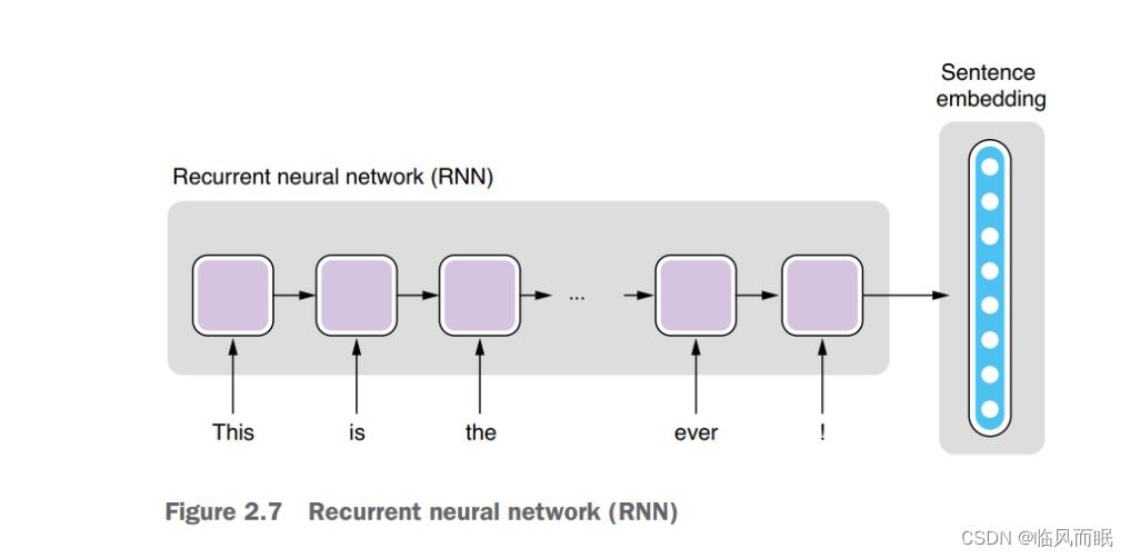
A recurrent neural network (RNN) is a neural network with loops, as shown in figure 2.7. It has an internal structure that is applied to the input again and again. Using the programming analogy(类比), it’s like writing a function that contains for word in sentence: that loops over each word in the input sentence. It can either output the interim values of the internal variables of the loop, or the final values of the variables after the loop is finished, or both. If you just take the final values, you can use an RNN as a function that transforms a sentence to a vector with a fixed length.
In many NLP tasks, you can use an RNN to transform a sentence to an embedding of the sentence. Remember word embeddings? They were fixed-length representation of words. Similarly, RNNs can produce fixed-length representation of sentences.
linear layers
-
Another type of neural network component we’ll be using here is linear layers. A linear layer, also called a fully connected layer, transforms a vector to another vector in a linear fashion. As mentioned earlier, layer is just a fancier term(术语) for a substructure of neural networks, because you can stack them on top of each other to form a larger structure.
-
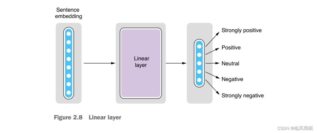
Neural networks can learn nonlinear relationships between the input and the output. Why would we want something that is more constrained (linear) at all? Linear layers are used for compressing (or less often, expanding) vectors by reducing (or increasing) the dimensionality. For example, assume you receive a 64- dimensional vector (an array of 64 float numbers) from an RNN as a sentence embedding, but all you care about is a smaller number of values that are essential for your prediction. In sentiment analysis, you may care about only five values that correspond to five different sentiment labels, namely, strongly positive, positive, neutral, negative, and strongly negative. But you have no idea how to extract those five values from the embedded 64 values. This is exactly where a linear layer comes in handy—you can add a layer that transforms a 64-dimensional vector to a 5-dimensional one, and the neural networks figure out how to do that well.
2.4.3 Architecture for sentiment analysis
Now you are ready to put the components together to build the neural network for the sentiment analyzer. First, you need to create the RNN as follows:
# Seq2VecEncoder is a neural network abstraction that takes a sequence of something
# (usually a sequence of embedded word vectors), processes it, and returns a single
# vector. Oftentimes this is an RNN-based architecture (e.g., LSTM or GRU), but
# AllenNLP also supports CNNs and other simple architectures (for example,
# just averaging over the input vectors).
encoder = PytorchSeq2VecWrapper(
    torch.nn.LSTM(EMBEDDING_DIM, HIDDEN_DIM, batch_first=True))
Here, you are creating an RNN (or more specifically, one type of RNN called LSTM, which stands for long short-term memory). The size of the input vector is EMBEDDING_DIM, which we saw earlier, and that of the output vector is HIDDEN_DIM.
Next, you need to create a linear layer, as shown here:
self.linear = torch.nn.Linear(in_features=encoder.get_output_dim(),
                                      out_features=vocab.get_vocab_size('labels'))
The size of the input vector is defined by in_features, whereas out_features is that of the output vector. Because we are transforming the sentence embedding to a vector whose elements correspond to five sentiment labels, we need to specify the size of the encoder output and obtain the total number of labels from vocab.
Finally, we can connect those components and build a model as shown in the following code.
code Building a sentiment analyzer model
class LstmClassifier(Model):
 def __init__(self,
              word_embeddings: TextFieldEmbedder,
              encoder: Seq2VecEncoder,
              vocab: Vocabulary,
              positive_label: str = '4') -> None:
         super().__init__(vocab)
         self.word_embeddings = word_embeddings
         self.encoder = encoder
         self.linear = torch.nn.Linear(in_features=encoder.get_output_dim(),
		out_features=vocab.get_vocab_size('labels'))
 		 self.loss_function = torch.nn.CrossEntropyLoss()
 def forward(self,
             tokens: Dict[str, torch.Tensor],
             label: torch.Tensor = None) -> torch.Tensor:
     mask = get_text_field_mask(tokens)
     embeddings = self.word_embeddings(tokens)
     encoder_out = self.encoder(embeddings, mask)
     logits = self.linear(encoder_out)
 	 output = "logits": logits
     if label is not None:
     	self.accuracy(logits, label)
     	self.f1_measure(logits, label)
     	output["loss"] = self.loss_function(logits, label)
     return output
- 这里面的
forward()function- the most important function that every neural network model has. Its role is to take the input, pass it through subcomponents of the neural network, and produce the output. Although the function has some unfamiliar logics that we haven’t covered yet (such as mask and loss), what’s important here is the fact that you can chain(链接) the subcomponents of the model (word embeddings, RNN, and the linear layer) as if they were functions that transform the input (tokens), and you get something called logits at the end of the pipeline. Logit is a term in statistics that has a specific meaning, but here, you can think of it as something like a score for a class. The higher the score is for a specific label, the more confident that the label is the correct one.
2.5 Loss functions and optimization
-
How can we make it so that neural networks produce the output that we actually want?
-
Neural networks are not just like regular functions that you usually write in programming languages. They are trainable, meaning that they can receive some feedback and change their internal parameters so that they can produce more accurate outputs, even for the same inputs next time around.
-
Notice there are two parts to this— receiving feedback and adjusting parameters, which are done through loss functions and optimization.
-
A
loss functionis a function that measures how far an output of a machine learning model is from a desired one. -
The difference between an actual output and a desired one is called the
loss. Loss is also calledcostin some contexts. Either way, the bigger the loss, the worse it is, and you want it as close to zero as possible. Take sentiment analysis, for example. If the model thinks a sentence is 100% negative, but the training data says it’s strongly positive, the loss will be big. On the other hand, if the model thinks a sentence is maybe 80% negative and the training label is indeed negative, the loss will be small. It will be zero if both match exactly. -
PyTorch provides a wide range of functions to compute losses. What we need here is called
cross-entropy loss, which is often used for classification problems, as shown here:self.loss_function = torch.nn.CrossEntropyLoss()It can be used later by passing a prediction and labels from the training set as follows:
output["loss"] = self.loss_function(logits, label)Then, this is where the magic happens. Neural networks, thanks to their mathematical properties, know how to change their internal parameters to make the loss smaller. Upon receiving some large loss, the neural network goes, “Oops, sorry, that was my mistake, but I’ll do better next round!” (hhh这里写的很好玩) and changes its parameters. Remember I talked about a function that you write in a programming language that has some magic constants in it? Neural networks act like that function but know exactly how to change the magic constants to reduce the loss.
They do this for each and every instance in the training data, so that they can produce more correct answers for as many instances as possible. Of course, they can’t reach the perfect answer after adjusting the parameters only once. It requires multiple passes, called
epochs, over the training data.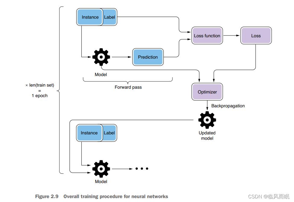
-
The process where a neural network computes an output from an input using the current set of parameters is called the
forward pass. The way the loss is fed back to the neural network is calledbackpropagation. An algorithm calledstochastic gradient descent (SGD)is often used to minimize the loss.The process where the loss is minimized is called
optimization, and the algorithm (such as SGD) used to achieve this is called theoptimizer. You can initialize an optimizer using PyTorch as follows:optimizer = optim.Adam(model.parameters()) -
Here, we are using one type of optimizer called Adam. There are many types of optimizers proposed in the neural network community, but the consensus is that there is no single optimization algorithm that works well for any problem, and you should be ready to experiment with multiple ones for your own problem.
-
OK, that was a lot of technical terms. You don’t need to know the details of those algorithms for now, but it’d be helpful if you learn just the terms and what they roughly mean.
code Pseudocode for the neural network training loop
- Note that there are two nested loops, one over epochs and another over instances.
MAX_EPOCHS = 100
model = Model()
for epoch in range(MAX_EPOCHS):
 for instance, label in train_set:
 prediction = model.forward(instance)
 loss = loss_function(prediction, label)
 new_model = optimizer(model, loss)
 model = new_model
2.6 Training your own classifier
- we are going to train our own classifier using AllenNLP’s training framework.
2.6.1 Batching
-
So far, I have left out one piece of detail—batching. We assumed that an optimization step happens for each and every instance, as you saw in the earlier pseudocode. In practice, however, we usually group a number of instances together and feed them to a neural network, updating model parameters per each group, not per each instance. We call this group of instances a
batch. -
Batching is a good idea for a couple of reasons.
- The first is stability. Any data is inherently(本质上) noisy. Your dataset may contain sampling and labeling errors. If you update your model parameters for every instance, and if some instances contain errors, the update is influenced too much by the noise. But if you group instances into batches and compute the loss for the entire batch, not for individual instances, you can “average out” small errors and the feedback to your model stabilizes.
- The second reason is speed. Training neural networks involves a huge number of arithmetic operations such as matrix additions and multiplications, and it is often done on GPUs (graphics processing units). Because GPUs are designed so that they can process a huge number of arithmetic operations in parallel, it is often efficient if you pass a large amount of data and process it at once instead of passing instances one by one. Think of a GPU as a factory overseas that manufactures products based on your specifications. Because factories are often optimized for manufacturing a small variety of products at a large quantity, and there is overhead in communicating and shipping products, it is more efficient if you make a small number of orders for manufacturing a large quantity of products instead of making a large number of orders for manufacturing a small quantity of products, even if you want the same quantity of products in total in either way.
It is easy to group instances into batches using AllenNLP. The framework uses PyTorch’s
DataLoaderabstraction, which takes care of receiving instances and returning batches. We’ll use aBucketBatchSamplerthat groups instances into buckets of similar lengthssampler = BucketBatchSampler(batch_size=32, sorting_keys=["tokens"]) train_data_loader = MultiProcessDataLoader(reader, train_path, batch_sampler=sampler) dev_data_loader = MultiProcessDataLoader(reader, dev_path, batch_sampler=sampler)The parameter
batch_sizespecifies the size of the batch (the number of instances in a batch). There is often a “sweet spot” in adjusting this parameter. It should be large enough to have any effect of the batching I mentioned earlier, but also small enough so that batches fit in the GPU memory, because factories have the maximum capacity of products they can manufacture at once.
2.6.2 Putting everything together
Now you are ready to train your sentiment analyzer. We assume that you already defined and initialized your model as follows:
model = LstmClassifier(word_embeddings, encoder, vocab)
AllenNLP provides the Trainer class, which acts as a framework for putting all the components together and managing the training pipeline, as shown here
trainer = GradientDescentTrainer(
 model=model,
 optimizer=optimizer,
 data_loader=train_data_loader,
 validation_data_loader=dev_data_loader,
 patience=10,
 num_epochs=20,
 cuda_device=-1)
trainer.train()
You provide the model, optimizer, iterator, train set, dev set, and the number of epochs you want to the trainer and invoke the train method. The last parameter, cuda_device, tells the trainer which device (CPU or GPU) to use to use for training. Here, we are explicitly using the CPU.
2.7 Evaluating your classifier
-
When training an NLP/ML model, you should always monitor how the loss changes over time. If the training is working as expected, you should see the loss decrease over time. It doesn’t always decrease each epoch, but it should decrease as a general trend, because this is exactly what you told the optimizer to do. If it’s increasing or showing weird values (such as NaN), it’s usually a sign that your model is too limiting or there’s a bug in your code.
-
In addition to the loss, it is important to monitor other evaluation metrics you care about in your task. Loss is a purely mathematical concept that measures the closeness between your model and the answer, but smaller losses do not always guarantee better performance in the NLP task.
-
You can use a number of evaluation metrics, depending on the nature of your NLP task, but some that you need to know no matter what task you are working on include accuracy, precision, recall, and F-measure. Roughly speaking, these metrics measure how precisely your model’s predictions match the expected answers defined by the dataset.
-
For now, it suffices to know that they are used to measure how good your classifier is
-
To monitor and report evaluation metrics during training using AllenNLP, you need to implement the
get_metrics()method in your model class, which returns a dict from metric names to their values, as shown next.def get_metrics(self, reset: bool = False) -> Dict[str, float]: return 'accuracy': self.accuracy.get_metric(reset), **self.f1_measure.get_metric(reset)self.accuracy and self.f1_measure are defined in
__init__()as follows:self.accuracy = CategoricalAccuracy() self.f1_measure = F1Measure(positive_index)When you run
trainer.train()with the metrics defined, you’ll see progress bars like these after every epoch: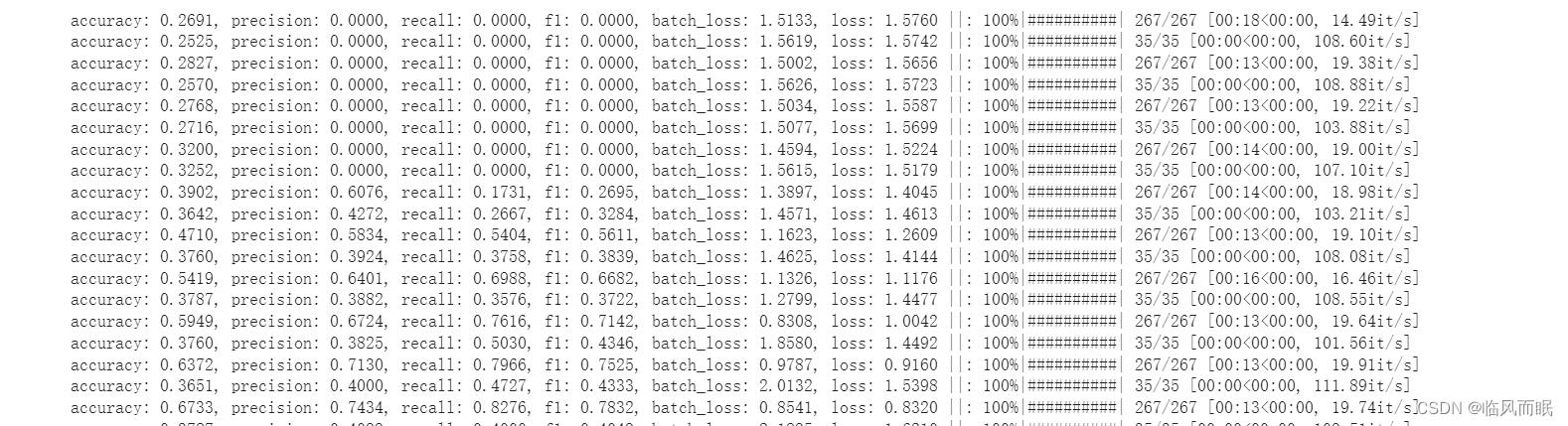
You can see that the training framework reports these metrics both for the train and the validation sets. This is useful not only for evaluating your model but also for monitoring the progress of the training. If you see any unusual values, such as extremely low or high numbers, you’ll know that something is wrong, even before the training completes.
-
You may have noticed a large gap between the train and the validation metrics.
-
Specifically, the metrics for the train set are a lot higher than those for the validation set. This is a common symptom of overfitting, where a model fits to a train set so well that it loses generalizability outside of it. This is why it’s important to monitor the metrics using a validation set as well, because you won’t know if it’s just doing well or overfitting only by looking at the training set metrics!
2.8 Deploying your application
The final step in making your own NLP application is deploying it. Training your model is only half the story. You need to set it up so that it can make predictions for new instances it has never seen. Making sure the model is serving predictions is critical in real-world NLP applications, and a lot of development efforts may go into this stage.
2.8.1 Making predictions
To make predictions for new instances your model has never seen (called test instances), you need to pass them through the same neural network pipeline as you did for training. It has to be exactly the same—otherwise, you’ll risk skewing the result. This is called training-serving skew(倾斜).
training-serving skew指的是训练和部署模型时出现的数据分布不一致的情况。这种情况可能会导致训练出的模型在真实环境中表现不佳。
AllenNLP provides a convenient abstraction called predictors, whose job it is to receive an input in its raw form (e.g., raw string), pass it through the preprocessing and neural network pipeline, and give back the result. I wrote a specific predictor for SST called SentenceClassifierPredictor, which you can call as follows
predictor = SentenceClassifierPredictor(model, dataset_reader=reader)
logits = predictor.predict('This is the best movie ever!')['logits']
Note that the predictor returns the raw output from the model, which is logits in this case. Remember, logits are some sort of scores corresponding to target labels, so if you want the predicted label itself, you need to convert it to the label. You don’t need to understand all the details for now, but this can be done by first taking the argmax of the logits, which returns the index of the logit with the maximum value, and then by looking up the label by the ID, as follows:
label_id = np.argmax(logits)
print(model.vocab.get_token_from_index(label_id, 'labels'))
If this prints out a “4,” congratulations! Label “4” corresponds to “very positive,” so your sentiment analyzer just predicted that the sentence “This is the best movie ever!” is very positive, which is indeed correct.
2.8.2 Serving predictions
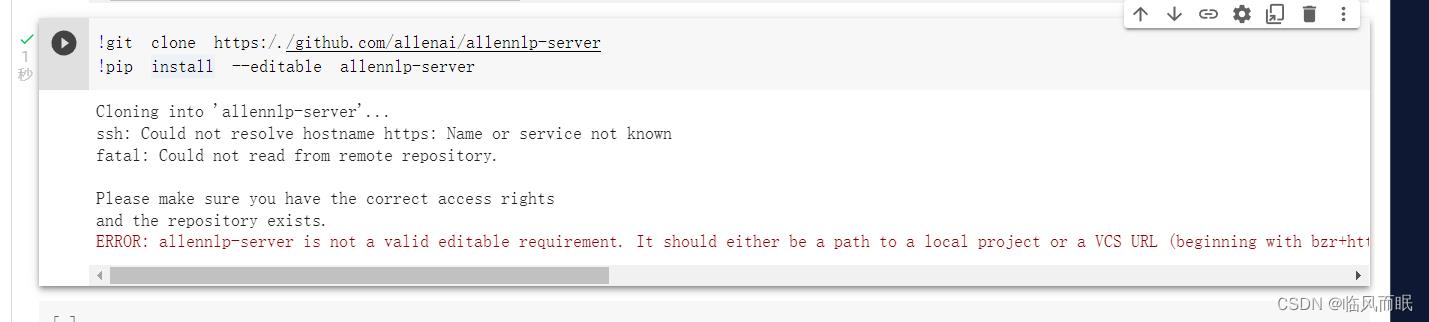
呃, colab里面好像搞不了
环境搭建
配环境挺头疼的,感觉pip那些基础知识还得夯实夯实
另外,codespace我好像每次都用的默认的, 它其实可以配置很多东西,之后再去探究
-
我先是在codespace给的默认环境里面
pip install allennlp==2.5.0,然后显示需要py3.6还有torch版本也不符合,于是我在终端里面创了个py版本是3.6的虚拟环境 RWNLP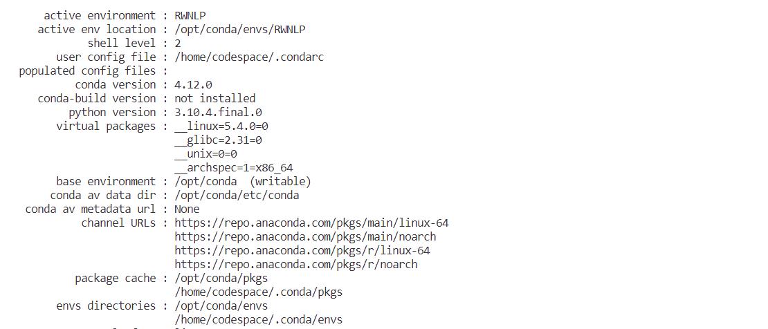
啊这,为啥
conda info显示出来的py是3.10捏… -
补充一下,激活之前首先需要在terminal里面输入
conda init bash,然后重启终端-
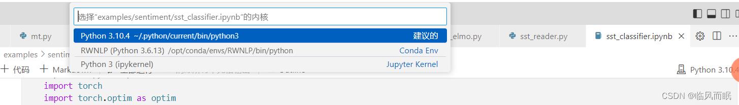
再打开激活
conda activate RWNLP然后就能在jupyter里面看到啦
-
上面的python版本我还是再verify一下,在终端输入
conda list python,问题不大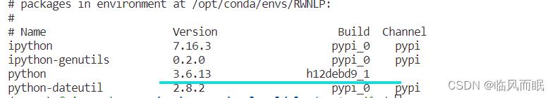
-
-
这一章需要使用allennlp
-
首先,什么是allennlp
AllenNLP is an open-source natural language processing library developed by the Allen Institute for Artificial Intelligence. It is built on PyTorch, a deep learning framework, and allows users to train and deploy state-of-the-art NLP models for tasks such as language translation, text classification, and questi
以上是关于情感分析入门demo《Real-World Natural Language Processing》 chap2:Your first NLP application的主要内容,如果未能解决你的问题,请参考以下文章
-