深度学习入门 2022 最新版 深度学习简介

Posted 2022-12-11 我是小白呀

【深度学习入门 2022 最新版】第一课 深度学习简介

• 概述
• 深度学习 vs 机器学习
• • 机器学习是什么
  • 深度学习是什么
  • 机器学习和深度学习的区别
• 神经网络
• • 机器学习实现二分类
  • 神经网络实现二分类
  • • TensorFlow
    • PyTorch
• 神经网络的原理
• • 张量
  • • 张量最小值 (补充)
    • 张量最大值 (补充)
  • 前向传播
  • 损失计算
  • 反向传播
  • 梯度下降
• 案例
• • 线性回归公式
  • 梯度下降
  • 完整代码

概述

该专栏为 2022 版深度学习入门教程. 学习此教程需要具备一定的 Python 基础知识和对机器学习的一些基础了解.

深度学习 vs 机器学习

机器学习是什么

机器学习 (Machine Learning) 能使机器自动从数据和过去的经验中学习. 通过模型在最少的人工干预下进行预测.

深度学习是什么

深度学习 (Deep Learning) 是机器学习的一种, 深度学习通过神经网络 (Neural Network), 对数据特征进行提取来实现数据的预测.

机器学习和深度学习的区别

举个例子, 我们需要对苹果和橘子进行分类.

机器学习的做法我们需要给模型提供量化的特征, 比如: 物体的重量, 物体的大小等. 但深度学习会通过神经网络 (Neural Network) 来自行提取特征. 因此, 深度学习所需要的算力要远远高于机器学习.

神经网络

神经网络 (Neural Network) 通过模拟人脑的运作方式来识别一组数据中的潜在关系. 如上面例子提到, 深度学习通过神经网络会自行提取多个特征, 类似我们发现苹果和橘子在大小, 重量上的区别, 组建一个由多个权重构成的网络. 神经网络可以适应不断变化的输入, 调整权重来获得最佳的结果.

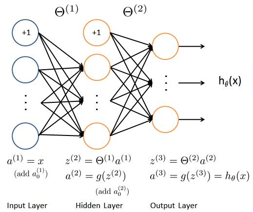
神经网络的组成部分:

• 输入层 (Input Layer): 输入层将初始数据代入神经网络, 供后续层神经元 (节点) 进行进一步处理. 比如, 图片识别中图片的像素, NLP 中的词向量
• 隐藏层 (Hidden Layer): 隐藏层帮助我们实现了特征提取, 隐藏层中的每一个节点对输入层对应不同的权重
• 输出层 (Output Layer): 输出层负责输出最后的结果

神经网络的每一层都有对应的神经网络与下一层连接.

机器学习实现二分类

机器学习实现橘子苹果分类 (数据是我编的, 表示重量和大小):

from sklearn.preprocessing import StandardScaler
from sklearn.linear_model import SGDClassifier
from sklearn.metrics import classification_report, mean_squared_error

def main():

    # 数据
    X_train = [[0.1, 0.2], [0.15, 0.22], [0.12, 0.21], [0.16, 0.22], [0.13, 0.2], [0.2, 0.39], [0.3, 0.45], [0.23, 0.4], [0.31, 0.44], [0.26, 0.4]]
    y_train =  [1, 1, 1, 1, 1, 0, 0, 0, 0, 0]
    X_test = [[0.11, 0.2], [0.12,0.22], [0.25, 0.4], [0.27, 0.41]]
    y_test =  [1, 1, 0, 0]

    # 标准化
    scaler = StandardScaler().fit(X_train)
    X_train = scaler.transform(X_train)
    X_test = scaler.transform(X_test)

    # 实例化SGD
    sgd = SGDClassifier()

    # 训练
    sgd.fit(X_train, y_train)

    # 预测
    y_predict = sgd.predict(X_test)

    # loss
    mse = mean_squared_error(y_test, y_predict)
    print("MSE:", mse)

    # 调试输出
    print(classification_report(y_test, y_predict))

if __name__ == '__main__':
    main()

输出结果:

MSE: 0.0
              precision    recall  f1-score   support

           0       1.00      1.00      1.00         2
           1       1.00      1.00      1.00         2

    accuracy                           1.00         4
   macro avg       1.00      1.00      1.00         4
weighted avg       1.00      1.00      1.00         4

神经网络实现二分类

TensorFlow

神经网络实现橘子苹果分类:

import tensorflow as tf

def main():
    # 定义超参数
    batch_size = 10  # 一次训练的样本数目
    iteration_num = 6  # 迭代次数
    learning_rate = 0.01  # 学习率
    optimizer = tf.keras.optimizers.Adam(learning_rate=learning_rate)  # 优化器
    loss = tf.losses.CategoricalCrossentropy(from_logits=True)  # 损失

    # 数据
    X_train = [[0.1, 0.2], [0.15, 0.22], [0.12, 0.21], [0.16, 0.22], [0.13, 0.2], [0.2, 0.39], [0.3, 0.45], [0.23, 0.4], [0.31, 0.44], [0.26, 0.4]]
    y_train =  [[1, 0], [1, 0], [1, 0], [1, 0], [1, 0], [0, 1], [0, 1], [0, 1], [0, 1], [0, 1]]
    X_test = [[0.11, 0.2], [0.12,0.22], [0.25, 0.4], [0.27, 0.41]]
    y_test =  [[1, 0], [1, 0], [0, 1], [0, 1]]


    model = tf.keras.Sequential([
        # 隐藏层
        tf.keras.layers.Dense(4, activation="relu"),

        # 输出层
        tf.keras.layers.Dense(2, activation="softmax")  # 2类 (苹果, 橘子)
    ])

    # 调试输出summary
    model.build(input_shape=[None, 2])  # 输入层
    print(model.summary())

    # 组合
    model.compile(optimizer=optimizer, loss=loss, metrics=["accuracy"])

    # 保存
    checkpoint = tf.keras.callbacks.ModelCheckpoint("model/model.h5", monitor='val_accuracy', verbose=1, save_best_only=True,
                                 mode='max')

    # 训练
    model.fit(X_train, y_train, validation_data=(X_test, y_test), epochs=iteration_num, batch_size=batch_size, callbacks=[checkpoint])



if __name__ == '__main__':
    main()

结果:

Model: "sequential"
_________________________________________________________________
Layer (type)                 Output Shape              Param #   
=================================================================
dense (Dense)                (None, 4)                 12        
_________________________________________________________________
dense_1 (Dense)              (None, 2)                 10        
=================================================================
Total params: 22
Trainable params: 22
Non-trainable params: 0
_________________________________________________________________
None
2022-11-18 18:42:25.102900: I tensorflow/compiler/mlir/mlir_graph_optimization_pass.cc:176] None of the MLIR Optimization Passes are enabled (registered 2)
2022-11-18 18:42:25.136804: I tensorflow/core/platform/profile_utils/cpu_utils.cc:114] CPU Frequency: 2301085000 Hz
Epoch 1/6
/root/miniconda3/envs/myconda/lib/python3.7/site-packages/tensorflow/python/keras/backend.py:4870: UserWarning: "`categorical_crossentropy` received `from_logits=True`, but the `output` argument was produced by a sigmoid or softmax activation and thus does not represent logits. Was this intended?"
  '"`categorical_crossentropy` received `from_logits=True`, but '
1/1 [==============================] - 0s 465ms/step - loss: 0.6889 - accuracy: 0.5000 - val_loss: 0.6872 - val_accuracy: 0.7500

Epoch 00001: val_accuracy improved from -inf to 0.75000, saving model to model/model.h5
Epoch 2/6
1/1 [==============================] - 0s 22ms/step - loss: 0.6873 - accuracy: 0.6000 - val_loss: 0.6857 - val_accuracy: 1.0000

Epoch 00002: val_accuracy improved from 0.75000 to 1.00000, saving model to model/model.h5
Epoch 3/6
1/1 [==============================] - 0s 33ms/step - loss: 0.6858 - accuracy: 1.0000 - val_loss: 0.6842 - val_accuracy: 1.0000

Epoch 00003: val_accuracy did not improve from 1.00000
Epoch 4/6
1/1 [==============================] - 0s 33ms/step - loss: 0.6842 - accuracy: 1.0000 - val_loss: 0.6828 - val_accuracy: 1.0000

Epoch 00004: val_accuracy did not improve from 1.00000
Epoch 5/6
1/1 [==============================] - 0s 32ms/step - loss: 0.6827 - accuracy: 1.0000 - val_loss: 0.6813 - val_accuracy: 1.0000

Epoch 00005: val_accuracy did not improve from 1.00000
Epoch 6/6
1/1 [==============================] - 0s 25ms/step - loss: 0.6812 - accuracy: 1.0000 - val_loss: 0.6799 - val_accuracy: 1.0000

Epoch 00006: val_accuracy did not improve from 1.00000

PyTorch

代码:

import torch
import torchvision
import torch.nn.functional as F
from torch.utils.data import DataLoader, TensorDataset
from torchsummary import summary



def train(model, optimizer, epoch, train_loader, use_cuda):
    """训练"""

    # 训练模式
    model.train()

    # 迭代
    for step, (x, y) in enumerate(train_loader):
        # 加速
        if use_cuda:
            model = model.cuda()
            x, y = x.cuda(), y.cuda()

        # 梯度清零
        optimizer.zero_grad()
        
        # 获得模型输出
        output = model(x)

        # 计算损失
        loss = F.cross_entropy(output, y)

        # 反向传播
        loss.backward()

        # 更新梯度
        optimizer.step()

        # 打印损失
        if step % 10 == 0:
            print('Epoch: , Step , Loss: '.format(epoch, step, loss))



def test(model, test_loader, use_cuda):
    """测试"""

    # 测试模式
    model.eval()

    # 存放正确个数
    correct = 0

    with torch.no_grad():
        for x, y in test_loader:

            # 加速
            if use_cuda:
                model = model.cuda()
                x, y = x.cuda(), y.cuda()

            # 获取结果
            output = model(x)

            # 预测结果
            pred = output.argmax(dim=1, keepdim=True)

            # 计算准确个数
            correct += pred.eq(y.view_as(pred)).sum().item()

    # 计算准确率
    accuracy = correct / len(test_loader.dataset) * 100

    # 输出准确
    print("Test Accuracy: %".format(accuracy))

    
def main():
    # 数据
    X_train = [[0.1, 0.2], [0.15, 0.22], [0.12, 0.21], [0.16, 0.22], [0.13, 0.2], [0.2, 0.39], [0.3, 0.45], [0.23, 0.4], [0.31, 0.44], [0.26, 0.4]]
    y_train =  [1, 1, 1, 1, 1, 0, 0, 0, 0, 0]
    X_test = [[0.11, 0.2], [0.12,0.22], [0.25, 0.4], [0.27, 0.41]]
    y_test =  [1, 1, 0, 0]

    
    
    network = torch.nn.Sequential(
        torch.nn.Linear(2, 4),
        torch.nn.Linear(4, 2),
    )
    
    # 定义超参数
    batch_size = 10  # 一次训练的样本数目
    iteration_num = 6  # 迭代次数
    learning_rate = 0.01  # 学习率
    optimizer = optim.Adam(network.parameters(), lr=learning_rate)  # 优化器
    
    # GPU 加速
    use_cuda = torch.cuda.is_available()

    if use_cuda:
        network.cuda()
    print("是否使用 GPU 加速:", use_cuda)
    print(summary(network, (10, 2)))  # 调试输出模型

    
    
    # 创建 DataLoader
    train_loader = DataLoader(TensorDataset(torch.tensor(X_train),torch.tensor(y_train)),batch_size=batch_size)
    test_loader = DataLoader(TensorDataset(torch.tensor(X_test),torch.tensor(y_test)),batch_size=batch_size)
    

    
    # 迭代
    for epoch in range(iteration_num):
        print("\\n================ epoch:  ================".format(epoch))
        train(network, optimizer, epoch, train_loader, use_cuda)
        test(network, test_loader, use_cuda)


if __name__ == '__main__':
    main()

输出结果:

是否使用 GPU 加速: False
----------------------------------------------------------------
        Layer (type)               Output Shape         Param #
================================================================
            Linear-1                [-1, 10, 4]              12
            Linear-2                [-1, 10, 2]              10
================================================================
Total params: 22
Trainable params: 22
Non-trainable params: 0
----------------------------------------------------------------
Input size (MB): 0.00
Forward/backward pass size (MB): 0.00
Params size (MB): 0.00
Estimated Total Size (MB): 0.00
----------------------------------------------------------------
None

================ epoch: 0 ================
Epoch: 0, Step 0, Loss: 0.6916642189025879
Test Accuracy: 50.0%

================ epoch: 1 ================
Epoch: 1, Step 0, Loss: 0.6879175305366516
Test Accuracy: 50.0%

================ epoch: 2 ================
Epoch: 2, Step 0, Loss: 0.6845822334289551
Test Accuracy: 50.0%

================ epoch: 3 ================
Epoch: 3, Step 0, Loss: 0.6816409826278687
Test Accuracy: 50.0%

================ epoch: 4 ================
Epoch: 4, Step 0, Loss: 0.679047703742981
Test Accuracy: 100.0%

================ epoch: 5 ================
Epoch: 5, Step 0, Loss: 0.6767345666885376
Test Accuracy: 100.0%

神经网络的原理

神经网络的工作流程:

1. 参数随机初始化
2. 前向传播
3. 损失计算
4. 反向传播
5. 梯度下降
6. 重复 2-5 步, 直到指定迭代次数

张量

张量 (Tensor) 是深度学习经常提到的一个词, 张量实际上代表的就是一个多维数组. 张量的目的是能够妆造更高维度的矩阵 & 向量.

1 维张量 = 1 维数组
2 维张量 = 2 维数组
3 维张量 = 3 维数组

张量最小值 (补充)

reduce_min函数可以帮助我们计算一个张量各个维度上元素的最小值. (补充, 了解即可, 后面会具体详解)

格式:

tf.math.reduce_min(
    input_tensor, axis=None, keepdims=False, name=None
)

参数:

• input_tensor: 传入的张量
• axis: 维度, 默认计算所有维度
• keepdims: 如果为真保留维度, 默认为 False
• name: 数据名称

张量最大值 (补充)

reduce_max函数可以帮助我们计算一个张量各个维度上元素的最大值. (补充, 了解即可, 后面会具体详解)

格式:

tf.math.reduce_max(
    input_tensor, axis=None, keepdims=False, name=None
)

参数:

• input_tensor: 传入的张量
• axis: 维度, 默认计算所有维度
• keepdims: 如果为真保留维度, 默认为 False
• name: 数据名称

前向传播

前向传播 (Forward Propagation) 是将上一层输出作为下一层的输入. 并计算下一层的输出, 一直运算到输出层为止.

如图:

mnist 训练代码片段 (前向传播):

def train(epoch):  # 训练
    for step, (x, y) in enumerate(train_db):  # 每一批样本遍历
        # 把x平铺 [256, 28, 28] => [256, 784]
        x = tf.reshape(x, [-1, 784])

        with tf.GradientTape() as tape:  # 自动求解
            # 第一个隐层 [256, 784] => [256, 256]
            # [256, 784]@[784, 256] + [256] => [256, 256] + [256] => [256, 256] + [256, 256] (广播机制)
            h1 = x @ w1 + tf.broadcast_to(b1, [x.shape[0], 256])
            h1 = tf.nn.relu(h1)  # relu激活

            # 第二个隐层 [256, 256] => [256, 128]
            h2 = h1 @ w2 + b2
            h2 = tf.nn.relu(h2)  # relu激活

            # 输出层 [256, 128] => [128, 10]
            out = h2 @ w3 + b3

            # 计算损失MSE(Mean Square Error)
            y_onehot = tf.one_hot(y, depth=10)  # 转换成one_hot编码
            loss = tf.square(y_onehot - out)  # 计算总误差
            loss = tf.reduce_mean(loss)  # 计算平均误差MSE

损失计算

损失函数 (Loss Function), 又称为代价函数, 用于计算模型输出值和真实值之间的差距. 通过减小损失, 我们可以让模型的输入与真实值更接近.

损失函有很多种, 在后续的章节中会详细说明, 在本节中就讲一个最简单的损失函数 MSE. 平方差 (Mean Square Error, MSE), 即计算两个值之间平方的差.

公式如下:

$MSE=\frac{1}{N}{\sum }_{i=1}^n(Y_i-Y_i^{{}^{\prime }})$

反向传播

反向传播 (Back Propagation) 会计算损失函数的梯度, 反馈给模型. 然后模型进行梯度下降, 更新权重, 从而最小化损失.

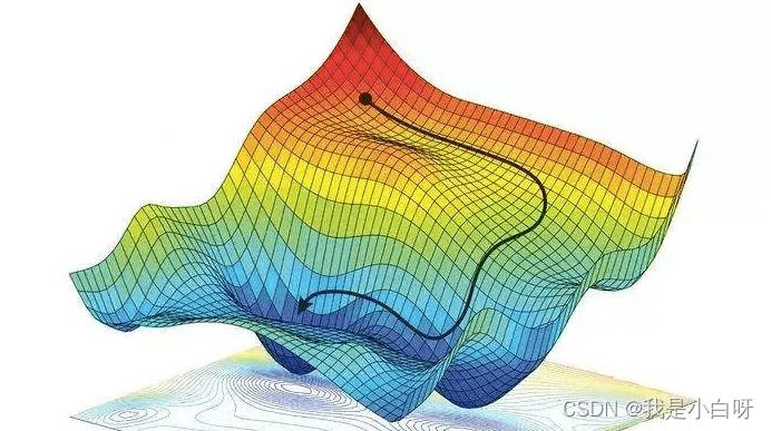
梯度下降

梯度下降 (Gradient Descent) 用于迭代模型的权重, 用于找到模型损失的最小值.

案例

下面我们通过一个线性回归 (Linear Regression) 来详解一下以上的神经网络工作流程.

线性回归公式

$y=w\times x+b$

• w: weight, 权重系数
• b: bias, 偏置顶
• x: 特征值
• y: 预测值

梯度下降

$w^{\prime }=w-lr\times \frac{dloss}{dw}$

$\frac{dloss}{dw}=\frac{1}{N}{\sum }_{i=1}^n(w\times x+b{)}^2{}^{\prime }$

$\frac{dloss}{dw}=\frac{2}{N}{\sum }_{i=1}^{n}x(w\times x+b)$

• w: weight, 权重参数
• w’: 更新后的 weight
• lr : learning rate, 学习率
• dloss/dw: 损失函数对 w 求导

$b^{\prime }=b-lr\times \frac{dloss}{db}$

$\frac{dloss}{db}=\frac{1}{N}{\sum }_{i=1}^n(w\times x+b{)}^2{}^{\prime }$

$\frac{dloss}{db}=\frac{2}{N}{\sum }_{i=1}^n(w\times x+b)$

• w: weight, 权重参数
• w’: 更新后的 weight
• lr : learning rate, 学习率
• dloss/dw: 损失函数对 b 求导

完整代码

代码:

import numpy as np
import pandas as pd
import tensorflow as tf


def run():
    """
    主函数
    :return: 无返回值
    """

    # 生成随机数据
    data = pd.DataFrame(np.random.randint(1, 100, size=(50, 2)))

    # 定义超参数
    learning_rate = 0.00002  # 学习率
    w_initial = 0  # 权重初始化
    b_initial = 0  # 偏置顶初始化
    w_end = 0  # 存放返回结果
    b_end = 0  # 存放返回结果
    num_interations = 50  # 迭代次数

    # 调试输出初始误差
    print("Starting gradient descent at w = , b = , error = "
          .format(w_initial, b_initial, calculate_MSE(w_initial, b_initial, data)))
    print("Running...")

    # 得到训练好的值
    w_end, b_end = runner(w_initial, b_initial, data, learning_rate, num_interations, )

    # 调试输出训练后的误差
    print("\\nAfter  iterations w = , b = , error = "
          .format(num_interations, w_end, b_end, calculate_MSE(w_end, b_end, data)))


def calculate_MSE(w, b, points):
    """
    计算误差MSE
    :param w: weight, 权重
    :param b: bias, 偏置顶
    :param points: 数据
    :return: 返回MSE (Mean Square Error)
    """

    total_error = 0  # 存放总误差, 初始化为0

    # 遍历数据
    for i in range(len(points)):
        # 取出x, y
        x = points.iloc[i, 0]  # 第一列
        y = points.iloc[i, 1]  # 第二列

        # 计算MSE
        total_error += (y - (w * x + b)) ** 2  # 计总误差
        MSE = total_error / len(points)  # 计算平均误差

    # 返回MSE
    return MSE


def step_gradient(index, w_current, b_current, points, learning_rate=0.0001):
    """
    计算梯度下降, 跟新权重
    :param index: 现行迭代编号
    :param w_current: weight, 权重
    :param b_current: bias, 偏置顶
    :param points: 数据
    :param learning_rate: lr, 学习率 (默认值: 0.0001)
    :return: 返回跟新过后的参数数组
    """

    b_gradient = 0  # b的导, 初始化为0
    w_gradient = 0  # w的导, 初始化为0
    N = len(points)  # 数据长度

    # 遍历数据
    for i in range(len(points)):
        # 取出x, y
        x = points.iloc[i, 0]  # 第一列
        y = points.iloc[i, 1]  # 第二列

        # 计算w的导, w的导 = 2x(wx+b-y)
        w_gradient += (2 / N) * x * ((w_current * x + b_current) - y)

        # 计算b的导, b的导 = 2(wx+b-y)
        b_gradient += (2 / N) * ((w_current * x + b_current) - y)

    # 跟新w和b
    w_new = w_current - (learning_rate * w_gradient)  # 下降导数*学习率
    b_new = b_current - (learning_rate * b_gradient)  # 下降导数*学习率

    # 每迭代10次, 调试输出
    if index % 10 == 0:
        print("This is the th iterations w = , b = , error = "
              .format(index, w_new, b_new,
                      calculate_MSE(w_new, b_new, points)))

    # 返回更新后的权重和偏置顶
    return [w_new, b_new]


def runner(w_start, b_start, points, learning_rate, num_iterations):
    """
    迭代训练
    :param w_start: 初始weight
    :param b_start: 初始bias
    :param points: 数据
    :param learning_rate: 学习率
    :param num_iterations: 迭代次数
    :return: 训练好的权重和偏执顶
    """

    # 定义w_end, b_end, 存放返回权重
    w_end = w_start
    b_end = b_start

    # 更新权重
    for i in range(1, num_iterations + 1):
        w_end, b_end = step_gradient(i, w_end, b_end, points, learning_rate)

    # 返回训练好的b, w
    return [w_end, b_end]


if __name__ == "__main__":  # 判断是否为直接运行
    # 执行主函数
    run()

输出结果:

Starting gradient descent at w = 0, b = 0, error = 2876.62
Running...
This is the 10th iterations w = 0.5460298230246148, b = 0.011931377672111465, error = 1240.3922367823025
This is the 20th iterations w = 0.6674152889847551, b = 0.017605573881127178, error = 1159.399196042907
This is the 30th iterations w = 0.6943653427274579, b = 0.02188796060553594, error = 1155.3218750586157
This is the 40th iterations w = 0.7003141856782037, b = 0.02586053371750557, error = 1155.0485126940196
This is the 50th iterations w = 0.7015926351060051, b = 0.02976391514280423, error = 1154.9632928699962

After 50 iterations w = 0.7015926351060051, b = 0.02976391514280423, error = 1154.9632928699962