使用 OpenCV 测量图像中对象之间的距离

Posted 2022-09-29 AI浩

现在，我们已经完成了关于测量图像中对象的大小和计算对象之间的距离的三部分系列的最后一部分。
两周前，我们通过学习如何（正确地）使用 Python 和 OpenCV 以顺时针方式对坐标进行排序，开始了这一轮教程。 然后，上周，我们讨论了如何使用参考对象测量图像中对象的大小。
这个引用对象应该有两个重要的属性，包括：
1 我们知道物体的尺寸（以英寸、毫米等为单位）。
2 它可以在我们的图像中轻松识别（基于位置或外观）。
给定这样一个参考对象，我们可以使用它来计算图像中对象的大小。
今天，我们将结合本系列之前的博客文章中使用的技术，并使用这些方法来计算对象之间的距离。

使用 OpenCV 测量图像中对象之间的距离

计算对象之间的距离与计算图像中对象的大小非常相似——这一切都从参考对象开始。
正如我们之前的博客文章中所详述的，我们的引用对象应该有两个重要的属性：

• 属性#1：我们知道物体的尺寸，单位是一些可测量的单位（如英寸、毫米等）。
• 属性 #2：我们可以轻松找到并识别图像中的参考对象。
  就像我们上周所做的那样，我们将使用美国 25 美分作为参考对象，其宽度为 0.955 英寸（满足属性 #1）。
  我们还将确保我们的四分之一始终是我们图像中最左边的对象，从而满足属性#2：

我们在这张图片中的目标是（1）找到四分之一，然后（2）使用四分之一的尺寸来测量四分之一和所有其他对象之间的距离。

定义我们的参考对象和计算距离

让我们继续开始这个例子。 打开一个新文件，将其命名为 distance_between。 py ，并插入以下代码：

# import the necessary packages
from scipy.spatial import distance as dist
from imutils import perspective
from imutils import contours
import numpy as np
import argparse
import imutils
import cv2


def midpoint(ptA, ptB):
    return ((ptA[0] + ptB[0]) * 0.5, (ptA[1] + ptB[1]) * 0.5)


# construct the argument parse and parse the arguments
ap = argparse.ArgumentParser()
ap.add_argument("-i", "--image", required=True, help="path to the input image")
ap.add_argument("-w", "--width", type=float, required=True,
                help="width of the left-most object in the image (in inches)")
args = vars(ap.parse_args())

我们这里的代码与上周几乎相同。 我们首先在第 2-8 行导入所需的 Python 包。 如果你还没有安装 imutils 包，现在停止安装它：

pip install imutils

否则，您应该在撰写本文时升级到最新版本 0.3 .6），以便您拥有更新的 order_points 函数：

pip install --upgrade imutils

第 14-19 行解析我们的命令行参数。 我们这里需要两个开关：image，这是包含我们要测量的对象的输入图像的路径，以及 --width，我们的参考对象的宽度（以英寸为单位）。
接下来，我们需要对图像进行预处理：

# load the image, convert it to grayscale, and blur it slightly
image = cv2.imread(args["image"])
gray = cv2.cvtColor(image, cv2.COLOR_BGR2GRAY)
gray = cv2.GaussianBlur(gray, (7, 7), 0)
# perform edge detection, then perform a dilation + erosion to close gaps in between object edges
edged = cv2.Canny(gray, 50, 100)
edged = cv2.dilate(edged, None, iterations=1)
edged = cv2.erode(edged, None, iterations=1)
# find contours in the edge map
cnts = cv2.findContours(edged.copy(), cv2.RETR_EXTERNAL, cv2.CHAIN_APPROX_SIMPLE)
cnts = imutils.grab_contours(cnts)
# sort the contours from left-to-right and, then initialize the distance colors and reference object
(cnts, _) = contours.sort_contours(cnts)
colors = ((0, 0, 255), (240, 0, 159), (0, 165, 255), (255, 255, 0), (255, 0, 255))
refObj = None

第 22-24 行从磁盘加载我们的图像，将其转换为灰度，然后使用具有 7×7 内核的高斯滤波器对其进行模糊处理。
一旦我们的图像被模糊，我们应用 Canny 边缘检测器来检测图像中的边缘 - 然后执行膨胀 + 腐蚀以关闭边缘图中的任何间隙（第 28-30 行）。

调用 cv2. findContours 检测边缘图中对象的轮廓（第 33-35 行），而第 39 行从左到右对我们的轮廓进行排序。 由于我们知道我们的美国四分之一（即参考对象）将始终是图像中最左侧的对象，因此从左到右对轮廓进行排序可确保与参考对象对应的轮廓始终是第一个条目 在cnts列表中。
然后，我们初始化用于绘制距离的颜色列表以及 ref0b j 变量，该变量将存储我们的边界框、质心和参考对象的每度量像素值。

# loop over the contours individually
for c in cnts:
    # if the contour is not sufficiently large, ignore it
    if cv2.contourArea(c) < 100: continue
    # compute the rotated bounding box of the contour
    box = cv2.minAreaRect(c)
    box = cv2.cv.BoxPoints(box) if imutils.is_cv2() else cv2.boxPoints(box)
    box = np.array(box, dtype="int")
    # order the points in the contour such that they appear
    #  in top-left, top-right, bottom-right, and bottom-left order,
    #  then draw the outline of the rotated bounding box
    box = perspective.order_points(box)
    #  compute the center of the bounding box
    cX = np.average(box[:, 0])
    cY = np.average(box[:, 1])

在第 45 行，我们开始循环遍历 cnts 列表中的每个轮廓。 如果轮廓不够大（47 和48行），我们忽略它。
否则，第 51-53 行计算当前对象的旋转边界框（OpenCV 2.4 使用 c v 2 . c v . BoxPoints ，OpenCV 3 使用 c v 2 . boxPoints ）。
在第 59 行调用 order_points 重新排列边界框 (x, y) - 左上角、右上角、右下角和左下角的坐标，正如我们将看到的，当我们转到 计算对象角之间的距离。
第 62 行和63行通过取边界框在 x 和 y 方向上的平均值来计算旋转边界框的中心 (x, y) 坐标。
下一步是校准我们的 refobj ：

    # if this is the first contour we are examining (i.e.,
    # the left-most contour), we presume this is the reference object
    if refObj is None:
        # unpack the ordered bounding box, then compute the
        #  midpoint between the top-left and top-right points,
        #  followed by the midpoint between the top-right and
        #  bottom-right
        (tl, tr, br, bl) = box
        (tlblX, tlblY) = midpoint(tl, bl)
        (trbrX, trbrY) = midpoint(tr, br)
        # compute the Euclidean distance between the midpoints,
        #  then construct the reference object
        D = dist.euclidean((tlblX, tlblY), (trbrX, trbrY))
        refObj = (box, (cX, cY), D / args["width"])
        continue

如果我们的 refobj是 None （68行），那么我们需要初始化它。
我们首先解包（有序）旋转的边界框坐标，并分别计算左上角和左下角之间的中点以及右上角和右下角点（第 73-75 行）。

从那里，我们计算点之间的欧几里得距离，为我们提供“每公制像素”，使我们能够确定有多少像素适合 -width 英寸。

注意：有关“pixels-permetric”变量的更详细讨论，请参阅上周的帖子。
最后，我们将 ref0b j 实例化为一个 3 元组，包括：
1 旋转后的边界框参考对象对应的排序坐标。
2 参考对象的质心。
3 我们将用于确定对象之间距离的每公制像素比率。
我们的下一个代码块处理在我们的参考对象和我们当前正在检查的对象周围绘制轮廓，然后构造 refCoords 和 objCoords，使得 (1) 边界框坐标和 (2) (x, y) 坐标的质心包含在相同的数组中：

    # draw the contours on the image
    orig = image.copy()
    cv2.drawContours(orig, [box.astype("int")], -1, (0, 255, 0), 2)
    cv2.drawContours(orig, [refObj[0].astype("int")], -1, (0, 255, 0), 2)
    # stack the reference coordinates and the object coordinates to include the object center
    refCoords = np.vstack([refObj[0], refObj[1]])
    objCoords = np.vstack([box, (cX, cY)])

我们现在准备计算图像中对象的各个角和质心之间的距离：

    # loop over the original points
    for ((xA, yA), (xB, yB), color) in zip(refCoords, objCoords, colors):
        # draw circles corresponding to the current points and connect them with a line    W
        cv2.circle(orig, (int(xA), int(yA)), 5, color, -1)
        cv2.circle(orig, (int(xB), int(yB)), 5, color, -1)
        cv2.line(orig, (int(xA), int(yA)), (int(xB), int(yB)), color, 2)
        # compute the Euclidean distance between the coordinates,
        # and then convert the distance in pixels to distance in units
        D = dist.euclidean((xA, yA), (xB, yB)) / refObj[2]
        (mX, mY) = midpoint((xA, yA), (xB, yB))
        cv2.putText(orig, ":.1fin".format(D), (int(mX), int(mY - 10)), cv2.FONT_HERSHEY_SIMPLEX, 0.55, color, 2)
        # show the output image
        cv2.imshow("Image", orig)
        cv2.waitKey(0)

在第94行上，我们开始循环通过对应于我们的参考对象和感兴趣的对象的（x，y） - 坐标。

然后，我们绘制一个代表当前点的（x，y） - 坐标的圆圈，我们正在计算并绘制一个线以连接点的距离（线97-110）。
从那里开始，第105行计算参考位置和对象位置之间的欧几里得距离，然后将距离除以“ Pixelsper-metric”，从而为我们提供了两个对象之间的最终距离。 然后在我们的图像上绘制计算距离（第106-108行）。

注意：对于左上，右上，右下，左下和质心坐标的每个距离计算，总共进行了五个距离的比较。
最后，第111和112行将输出图像显示到我们的屏幕上。

距离测量结果

要尝试我们的距离测量脚本，请使用本教程底部的“下载”表单将源代码和相应的图像下载到这篇文章。 将 . zip 文件，将目录更改为 distance_between。 py 脚本，然后执行以下命令：

 python distance_between. py --image images/example_01.png --width  0.955 

下面是演示脚本输出的 GIF 动画：

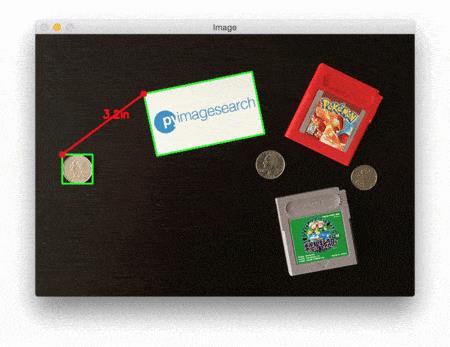
在每种情况下，我们的脚本都会匹配左上角（红色）、右上角（紫色）、右下角（橙色）、左下角（蓝绿色）和质心（粉红色）坐标，然后计算距离 （以英寸为单位）参考对象和当前对象之间的距离。
请注意图像中的两个四分之二完全平行，这意味着所有五个控制点之间的距离都是 6.1 英寸。
下面是第二个示例，这次计算我们的参考对象和一组药丸之间的距离：

python distance_between.py --image images/example_02.png --width 0.955

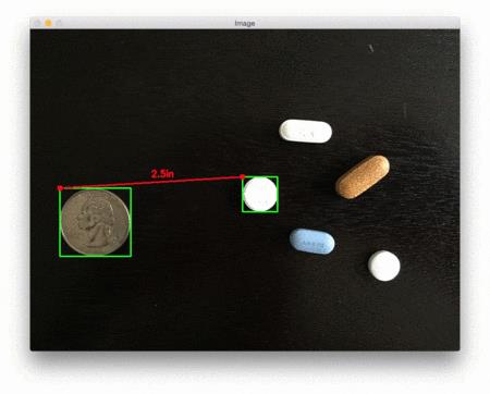
此示例可用作药丸分拣机器人的输入，该机器人自动取出一组药丸并根据它们的大小和与药丸容器的距离进行组织。

我们的最后一个示例计算我们的参考对象（一张 3.5 英寸 x 2 英寸的名片）与一组 $7^{\prime \prime }$ 黑胶唱片和一个信封之间的距离：

python distance_between.py --image images/example_03.png --width 3.5

总结

在我们关于测量对象尺寸系列的第三部分也是最后一部分中，我们学习了如何在图像中拍摄两个不同的对象，并以实际可测量的单位（例如英寸、毫米等）计算它们之间的距离。

正如我们在上周的帖子中发现的那样，在我们可以 (1) 计算对象的大小或 (2) 测量两个对象之间的距离之前，我们首先需要计算“像素/度量”比率，用于 确定有多少像素“适合”给定的测量单位。
一旦我们有了这个比率，计算物体之间的距离几乎是微不足道的。

完整代码

#!/usr/bin/env python
# -*- coding: UTF-8 -*-

# import the necessary packages
from scipy.spatial import distance as dist
from imutils import perspective
from imutils import contours
import numpy as np
import argparse
import imutils
import cv2


def midpoint(ptA, ptB):
    return ((ptA[0] + ptB[0]) * 0.5, (ptA[1] + ptB[1]) * 0.5)


# construct the argument parse and parse the arguments
ap = argparse.ArgumentParser()
ap.add_argument("-i", "--image", required=True, help="path to the input image")
ap.add_argument("-w", "--width", type=float, required=True,
                help="width of the left-most object in the image (in inches)")
args = vars(ap.parse_args())

# load the image, convert it to grayscale, and blur it slightly
image = cv2.imread(args["image"])
gray = cv2.cvtColor(image, cv2.COLOR_BGR2GRAY)
gray = cv2.GaussianBlur(gray, (7, 7), 0)
# perform edge detection, then perform a dilation + erosion to close gaps in between object edges
edged = cv2.Canny(gray, 50, 100)
edged = cv2.dilate(edged, None, iterations=1)
edged = cv2.erode(edged, None, iterations=1)
# find contours in the edge map
cnts = cv2.findContours(edged.copy(), cv2.RETR_EXTERNAL, cv2.CHAIN_APPROX_SIMPLE)
cnts = imutils.grab_contours(cnts)
# sort the contours from left-to-right and, then initialize the distance colors and reference object
(cnts, _) = contours.sort_contours(cnts)
colors = ((0, 0, 255), (240, 0, 159), (0, 165, 255), (255, 255, 0), (255, 0, 255))
refObj = None

# loop over the contours individually
for c in cnts:
    # if the contour is not sufficiently large, ignore it
    if cv2.contourArea(c) < 100: continue
    # compute the rotated bounding box of the contour
    box = cv2.minAreaRect(c)
    box = cv2.cv.BoxPoints(box) if imutils.is_cv2() else cv2.boxPoints(box)
    box = np.array(box, dtype="int")
    # order the points in the contour such that they appear
    #  in top-left, top-right, bottom-right, and bottom-left order,
    #  then draw the outline of the rotated bounding box
    box = perspective.order_points(box)
    #  compute the center of the bounding box
    cX = np.average(box[:, 0])
    cY = np.average(box[:, 1])

    # if this is the first contour we are examining (i.e.,
    # the left-most contour), we presume this is the reference object
    if refObj is None:
        # unpack the ordered bounding box, then compute the
        #  midpoint between the top-left and top-right points,
        #  followed by the midpoint between the top-right and
        #  bottom-right
        (tl, tr, br, bl) = box
        (tlblX, tlblY) = midpoint(tl, bl)
        (trbrX, trbrY) = midpoint(tr, br)
        # compute the Euclidean distance between the midpoints,
        #  then construct the reference object
        D = dist.euclidean((tlblX, tlblY), (trbrX, trbrY))
        refObj = (box, (cX, cY), D / args["width"])
        continue

    # draw the contours on the image
    orig = image.copy()
    cv2.drawContours(orig, [box.astype("int")], -1, (0, 255, 0), 2)
    cv2.drawContours(orig, [refObj[0].astype("int")], -1, (0, 255, 0), 2)
    # stack the reference coordinates and the object coordinates to include the object center
    refCoords = np.vstack([refObj[0], refObj[1]])
    objCoords = np.vstack([box, (cX, cY)])

    # loop over the original points
    for ((xA, yA), (xB, yB), color) in zip(refCoords, objCoords, colors):
        # draw circles corresponding to the current points and connect them with a line    W
        cv2.circle(orig, (int(xA), int(yA)), 5, color, -1)
        cv2.circle(orig, (int(xB), int(yB)), 5, color, -1)
        cv2.line(orig, (int(xA), int(yA)), (int(xB), int(yB)), color, 2)
        # compute the Euclidean distance between the coordinates,
        # and then convert the distance in pixels to distance in units
        D = dist.euclidean((xA, yA), (xB, yB)) / refObj[2]
        (mX, mY) = midpoint((xA, yA), (xB, yB))
        cv2.putText(orig, ":.1fin".format(D), (int(mX), int(mY - 10)), cv2.FONT_HERSHEY_SIMPLEX, 0.55, color, 2)
        # show the output image
        cv2.imshow("Image", orig)
        cv2.waitKey(0)