机器学习之TensorFlow - 补充学习中20220821

Posted 2022-08-24 lijiamin-

文章目录

• 前言
• 一、前置基础
• • 1.1 什么是神经网络
  • 1.2 什么是线性回归
  • 1.3 示例：识别手写数字
  • 1.4 示例：图像识别分类
  • 1.5 待定
  • 番外 Java/Python业务通信
• 二、待定
• 总结

前言

以下内容是在学习过程中的一些笔记，难免会有错误和纰漏的地方。如果造成任何困扰，很抱歉。

地址
关于TensorFlow | TensorFlow中文官网 (google.cn)

TensorFlow™是一个基于数据流编程（dataflow programming）的符号数学系统，是一个功能强大的开源软件库，它由Google的布莱恩（Brain）团队开发，被广泛应用于各类机器学习（machine learning）算法的编程实现，其前身是谷歌的神经网络算法库DistBelief。

一、前置基础

描述：这里可以添加本文要记录的大概内容

1.1 什么是神经网络

我们先从人类的大脑开始构思，人的大脑都是由无数个神经元构成，神经元之间相互通过脉络链接，组成一个庞大的神经元网络。

当人看到一只猫？抑或是一只狗时，神经网络会如何处理这些信息？

当一组图像输入到神经网络中，会被拆解成无数个可识别的/不可识别的标签，经过层层算法递进，找到最终自认为正确的一个结果（是猫是狗或是其它）。

神经网络小玩具地址
A Neural Network Playground (tensorflow.org)

然后简单的看一下分类

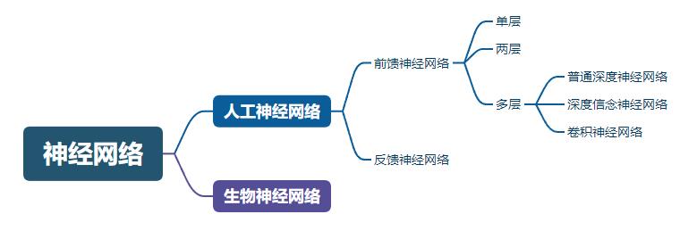
单个神经网络由多个互联的神经元构成，组织形式叫层，某一层的神经元会将消息传递到其下一层神经元（术语为“发射”），这即是神经网络的运行方式。

事实上，机器学习的模型就是一种计算函数的方法，这个函数把对应的输入映射到对应的输出上，在这个过程中，通过损失函数（待优化的内容）的一些度量指标，逐渐不断的将模型修正。

1.2 什么是线性回归

线性回归是利用数理统计中回归分析，来确定两种或两种以上变量间相互依赖的定量关系的一种统计分析方法，运用十分广泛。其表达形式为：

b为误差服从均值为0的正态分布。

如果只有一个自变量的情况下就叫一元回归；

如果有多个自变量的情况下就叫多元回归；

以你的工资为例，影响你工资的可能因素有很多：老板赏识、工作努力、运气不错等，如果从一个相对简单的角度去思考，你的工资仅仅由领导的心情决定，通过回归，我们就可以确定领导的心情（自变量：这类变量不依赖于其他任何变量）与工资（因变量：这类变量依赖于一个或多个自变量）之间的关系。

1.3 示例：识别手写数字

1

1

1.4 示例：图像识别分类

这个案例将训练一个神经网络模型，对运动鞋和衬衫等服装图像进行分类。

（1）数据准备及处理

首先导入相关的类库和数据集。

# TensorFlow and tf.keras
import tensorflow as tf
from tensorflow import keras

# Helper libraries
import numpy as np
import matplotlib.pyplot as plt

# 数据集导入
fashion_mnist = keras.datasets.fashion_mnist
(train_images, train_labels), (test_images, test_labels) = fashion_mnist.load_data()

该数据集包含 10 个类别的 70,000 个灰度图像。这些图像以低分辨率（28x28 像素）展示了单件衣物。

加载数据集会返回四个 NumPy 数组：

• train_images 和 train_labels 数组是训练集，即模型用于学习的数据；
• 测试集、test_images 和 test_labels 数组会被用来对模型进行测试；

我们针对这些标签进行一个简单的分类

# 将图像的标签分类
class_names = ['T-shirt/top', 'Trouser', 'Pullover', 'Dress', 'Coat',
               'Sandal', 'Shirt', 'Sneaker', 'Bag', 'Ankle boot']

标签	类
0	T恤/上衣
1	裤子
2	套头衫
3	连衣裙
4	外套
5	凉鞋
6	衬衫
7	运动鞋
8	包
9	短靴

# 浏览数据集
print(train_images.shape)
print(len(train_labels))
print(train_labels)

预处理数据 此时展示的是图像原始像素大小

# 预处理数据 此时展示的是图像原始像素大小
plt.figure()
plt.imshow(train_images[0])
plt.colorbar()
plt.grid(False)
plt.show()

需要将这些值缩小至0到1之间，然后将其馈送到神经网络模型

# 将这些值缩小至0到1之间 然后将其馈送到神经网络模型
train_images = train_images / 255.0
test_images = test_images / 255.0

# 验证数据的格式是否正确
plt.figure(figsize=(10, 10))
for i in range(25):
    plt.subplot(5, 5, i + 1)
    plt.xticks([])
    plt.yticks([])
    plt.grid(False)
    plt.imshow(train_images[i], cmap=plt.cm.binary)
    plt.xlabel(class_names[train_labels[i]])
plt.show()

（2）模型构建及训练

构建神经网络前

1. 配置模型的层；
2. 编译模型；

# 构建模型 -- 设置层
model = keras.Sequential([
    keras.layers.Flatten(input_shape=(28, 28)),
    keras.layers.Dense(128, activation='relu'),
    keras.layers.Dense(10)
])

第一层网络：keras.layers.Flatten，将图像格式从二维数组（28 x 28 像素）转换成一维数组（28 x 28 = 784 像素）。将该层视为图像中未堆叠的像素行并将其排列起来。

第二、三层网络：keras.layers.Dense，两层神经元序列。

# 编译模型
model.compile(optimizer='adam',
              loss=tf.keras.losses.SparseCategoricalCrossentropy(from_logits=True),
              metrics=['accuracy'])

# 训练模型
model.fit(train_images, train_labels, epochs=10)

# 评估准确率
test_loss, test_acc = model.evaluate(test_images, test_labels, verbose=2)
print('\\n 评估准确率 Test accuracy:', test_acc)

（3）预测/最终效果

这里我就偷懒一下吧

probability_model = tf.keras.Sequential([model,
                                         tf.keras.layers.Softmax()])
predictions = probability_model.predict(test_images)


# 效果查看
# predictions[0]
# test_labels[0]

# 图表绘制方法
def plot_image(i, predictions_array, true_label, img):
    predictions_array, true_label, img = predictions_array, true_label[i], img[i]
    plt.grid(False)
    plt.xticks([])
    plt.yticks([])

    plt.imshow(img, cmap=plt.cm.binary)

    predicted_label = np.argmax(predictions_array)
    if predicted_label == true_label:
        color = 'blue'
    else:
        color = 'red'

    plt.xlabel(" :2.0f% ()".format(class_names[predicted_label],
                                         100 * np.max(predictions_array),
                                         class_names[true_label]),
               color=color)


def plot_value_array(i, predictions_array, true_label):
    predictions_array, true_label = predictions_array, true_label[i]
    plt.grid(False)
    plt.xticks(range(10))
    plt.yticks([])
    thisplot = plt.bar(range(10), predictions_array, color="#777777")
    plt.ylim([0, 1])
    predicted_label = np.argmax(predictions_array)

    thisplot[predicted_label].set_color('red')
    thisplot[true_label].set_color('blue')


# 验证预测结果1
# i = 1
# plt.figure(figsize=(6, 3))
# plt.subplot(1, 2, 1)
# plot_image(i, predictions[i], test_labels, test_images)
# plt.subplot(1, 2, 2)
# plot_value_array(i, predictions[i], test_labels)
# plt.show()

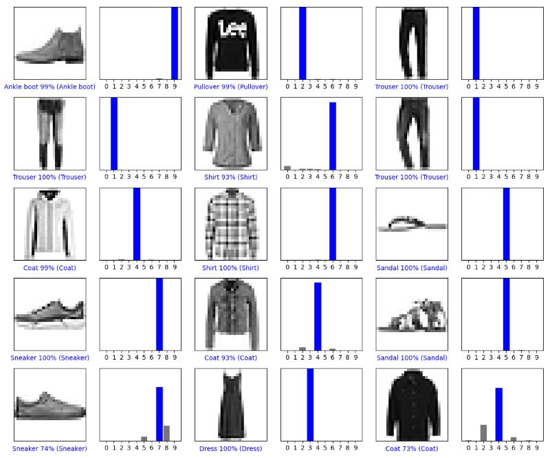
# 用模型的预测绘制几张图像
# Plot the first X test images, their predicted labels, and the true labels.
# Color correct predictions in blue and incorrect predictions in red.
num_rows = 5
num_cols = 3
num_images = num_rows * num_cols
plt.figure(figsize=(2 * 2 * num_cols, 2 * num_rows))
for i in range(num_images):
    plt.subplot(num_rows, 2 * num_cols, 2 * i + 1)
    plot_image(i, predictions[i], test_labels, test_images)
    plt.subplot(num_rows, 2 * num_cols, 2 * i + 2)
    plot_value_array(i, predictions[i], test_labels)
plt.tight_layout()
plt.show()

（4）完整代码

# TensorFlow and tf.keras
import tensorflow as tf
from tensorflow import keras

# Helper libraries
import numpy as np
import matplotlib.pyplot as plt

# 数据集导入 图像与标签 训练集与测试集
fashion_mnist = keras.datasets.fashion_mnist
(train_images, train_labels), (test_images, test_labels) = fashion_mnist.load_data()

# 将图像的标签分类
class_names = ['T-shirt/top', 'Trouser', 'Pullover', 'Dress', 'Coat',
               'Sandal', 'Shirt', 'Sneaker', 'Bag', 'Ankle boot']

# 将这些值缩小至0到1之间 然后将其馈送到神经网络模型
train_images = train_images / 255.0
test_images = test_images / 255.0

# 构建模型 -- 设置层
model = keras.Sequential([
    keras.layers.Flatten(input_shape=(28, 28)),
    keras.layers.Dense(128, activation='relu'),
    keras.layers.Dense(10)
])

# 编译模型
model.compile(optimizer='adam',
              loss=tf.keras.losses.SparseCategoricalCrossentropy(from_logits=True),
              metrics=['accuracy'])

# 训练模型
model.fit(train_images, train_labels, epochs=10)

# 评估准确率
test_loss, test_acc = model.evaluate(test_images, test_labels, verbose=2)
print('\\n 评估准确率 Test accuracy:', test_acc)

# 预测
probability_model = tf.keras.Sequential([model,
                                         tf.keras.layers.Softmax()])
predictions = probability_model.predict(test_images)


# 效果查看
# predictions[0]
# test_labels[0]

# 图表绘制方法
def plot_image(i, predictions_array, true_label, img):
    predictions_array, true_label, img = predictions_array, true_label[i], img[i]
    plt.grid(False)
    plt.xticks([])
    plt.yticks([])

    plt.imshow(img, cmap=plt.cm.binary)

    predicted_label = np.argmax(predictions_array)
    if predicted_label == true_label:
        color = 'blue'
    else:
        color = 'red'

    plt.xlabel(" :2.0f% ()".format(class_names[predicted_label],
                                         100 * np.max(predictions_array),
                                         class_names[true_label]),
               color=color)


def plot_value_array(i, predictions_array, true_label):
    predictions_array, true_label = predictions_array, true_label[i]
    plt.grid(False)
    plt.xticks(range(10))
    plt.yticks([])
    thisplot = plt.bar(range(10), predictions_array, color="#777777")
    plt.ylim([0, 1])
    predicted_label = np.argmax(predictions_array)

    thisplot[predicted_label].set_color('red')
    thisplot[true_label].set_color('blue')


# 验证预测结果1
# i = 1
# plt.figure(figsize=(6, 3))
# plt.subplot(1, 2, 1)
# plot_image(i, predictions[i], test_labels, test_images)
# plt.subplot(1, 2, 2)
# plot_value_array(i, predictions[i], test_labels)
# plt.show()

# 用模型的预测绘制几张图像
# Plot the first X test images, their predicted labels, and the true labels.
# Color correct predictions in blue and incorrect predictions in red.
num_rows = 5
num_cols = 3
num_images = num_rows * num_cols
plt.figure(figsize=(2 * 2 * num_cols, 2 * num_rows))
for i in range(num_images):
    plt.subplot(num_rows, 2 * num_cols, 2 * i + 1)
    plot_image(i, predictions[i], test_labels, test_images)
    plt.subplot(num_rows, 2 * num_cols, 2 * i + 2)
    plot_value_array(i, predictions[i], test_labels)
plt.tight_layout()
plt.show()

1.5 待定

1

番外 Java/Python业务通信

为什么会写下这一小节，因为我是一个Java开发，学习机器学习的目的是为了服务于我的业务系统，然而目前市面上大多数的系统都是基于Python/C++而研发的机器学习库，所以我也需要与时俱进，与他们进行结合。

1

1

二、待定

描述：这里可以添加本文要记录的大概内容

1

1

总结

提示：这里对文章进行总结：
例如：以上就是今天要讲的内容。